A Universal Simulation Platform for Flexible Systems

Please choose your JOURNAL, Vol. \volume? (\year?), pp. 1–11

Copyright © \pubyear? De Gruyter. DOI 10.1515/?????.\year?.\DOI?

A Universal Simulation Platform for Flexible Systems

Minh Hoang Vu,1,∗ Tajwar Abrar Aleef,1 Usama Pervaiz,1 Yeman Brhane Hagos1 and Saed Khawaldeh1

arXiv:1710.07186v1 [math.OC] 5 Oct 2017

1

Erasmus+ Joint Master Program in Medical Imaging and Applications University of Burgundy (France), University of Cassino (Italy) and University of Girona (Spain)

Abstract. This article proposes a universal simulation platform for simulating systems undergoing duress. In other words, this paper introduces a total simulation package which includes a number of methods of simulating the flexibility of a given system. This platform includes detailed procedures for simulating a flexible link by a numerical method called finite difference method. In order to verify the effectiveness of the proposed process, two examples are covered in different situations to discuss the importance of boundary control and mesh selection in the way of ensuring the stability of the system. In addition, a graphical user interface (GUI) application called the SimuFlex is designed having a selection of methods that the user can choose along with the parameters of the controllers that can be easily manipulated from the GUI.

Keywords. partial differential equations, finite difference method, flexible systems, simulation.

1 Introduction Flexible systems including strings and beams are widely applied in many areas of modern mechanical engineering [1], such as aerospace, civil [2], marine [3], chemical engineering [4], and especially in automatic manufacturing assembly. Systems with lightweight flexible links are becoming more popular as because they possess many advantages over the conventional rigid-link ones such as better speed, lower cost, greater labor productivity, enhanced machine efficiency, improved quality, increased system reliability, and reduced parts inventories to name a few. With the aim of improving industrial productivity, it is desirable to build systems with lightweight materials to increase the payload-to-weight ratio. This article is motivated by the industrial applications in the simulation of vibration of flexible structures. Corresponding author: Minh Hoang Vu, E-mail: [email protected]. Received: ???. Revised: ???. Accepted: ???.

Simulation is incredibly important as it helps to identify and solve problems before implementation. Furthermore, it can be used to predict the courses and results of certain actions, thus it enables to test hypotheses without having to carry them out in the practical world. Choosing a simulation method plays a key role in the successful simulation. Finite difference method (FDM) was chosen due to its simplicity and straightforward implementation. There are not many fast solvers and packages that are using FDM algorithm for partial difference equations (PDEs). Additionally, although Matlab provides a powerful visualization workspace, it does not have the functionality to allow researchers to input specifications and controller design at the same time. Engineers and researchers normally need to use a combination of tools for model building, controller design, and numerical simulation. Solving these difficulties greatly motivates the research in designing a GUI application, written on Matlab, for a complete system capable of simulating flexible-link systems. For the purpose of dynamic modeling and simulation, flexible systems are regarded as distributed parameter systems which are in infinite dimension with various boundary conditions involving functions of space and time. In practice, dynamics of flexible risers are mathematically represented by a set of PDEs with appropriate boundary equations or approximated by ordinary differential equations (ODEs). Since the vibration of flexible links are governed by PDEs, flexible systems are distributed-parameter and possess an infinite number of dimensions which makes them difficult to control[5]. Vibration reduction to minimize the disturbance effects is desirable for preventing damage and improving lifespan in industry. To avoid the vibration problem in a system, some popular methods, such as the application of point-care maps [6], variable structure control [7], sliding model control [8], energy-based robust control , model-free control [9], [10], distributed model predictive control [11], and boundary control [12] [13] are considered. In this article, both examples use boundary control. In this article, by using a well-understood numerical method, namely FDM, we design the boundary control based on the distributed parameter model of the flexible system. Then the importance of choosing appropriate control parameters can be discovered to improve the outcome of the final result. The main contribution of this article includes presenting a procedure for some kind of flexible systems represented by PDEs. Next, two examples are provided in order to demonstrate the procedure above. Finally, a GUI application, SimuFlex, for flexible systems is introduced.

2

Minh, Tajwar, Usama, Yeman and Saed

The rest of this article is organized as follows. Section 2 develops a procedure for simulating a flexible system using FDM. Section 3 shows two applications of the proposed process. Next, in Section 4, a GUI application, written by MATLAB for simulation of some specific flexible systems, is developed. Finally, Section 5 summarises and concludes the article.

respectively. Space and time grids have to be chosen appropriately but not too small or large because these selections might affect seriously the stability of the system. There must be a relationship between some crucial parameters, which assure the stability. This problem is discussed in the last part of this section.

2.3

2 Procedure for simulating a flexible system using finite difference method

Step 3: Apply boundary and initial conditions

Applying boundary and initial conditions in general equation in order to find a solution uniquely, which is invoked 2.1 Step 1: Modeling problem using Hamilton’s method from Keller’s theorem [15]. These conditions are comWith Lagrangian mechanics, Hamilton’s equations provide monly specified in terms of known values of the unknowns a new and equivalent way of looking at classical mechanics. on a part of the surface. These equations, however, do not provide a convenient way of solving particular problems. In addition, these equations provide deeper insights into both the general structure of 2.4 Step 4: Define general equation for each element classical mechanics and its connection to quantum mechanics as understood through Hamiltonian mechanics as well Substituting the derivatives with some finite difference foras its connection to remaining areas of science. mulas into the general equation for each point, thus we can Using Hamilton’s equations by following these steps obtain the algebraic system of equations. This method can [14]: be called the procedure of imposing the Dirichlet BCs [16]. (i) First write out the Lagrangian L = T − V . Express Some important finite difference approximation equations T and V as though you were going to use Lagrange’s are listed as follows [17]: equation.

(ii) Calculate the momenta by differentiating the Lagrangian with respect to velocity: pi (qi , q˙i , t) =

pL pq˙i

(1)

(iii) Express the velocities in terms of the momenta by inverting the expressions in step (ii). (iv) Compute the Hamiltonian using the usual definition of H as the Legendre transformation of L: H=

X i

X pL qi −L= q˙i pi − L pq˙i i

(2)

and then substitute for velocity in step (iii) (v) Apply Hamilton’s equations. Most likely, in step 1, researcher is expected to bring out governing equation, boundary initial conditions, disturbance, and controller of the system.

wt (i, j) =

w(i, j + 1) − w(i, j) + O(k) k

w(i, j + 1) − 2w(i, j) + w(i, j − 1) wtt (i, j) = + O(k 2 ) k2 wi (i, j) =

w(i + 1, j) − w(i, j) + O(h) h

w(i + 1, j) − 2w(i, j) + w(i − 1, j) wxx (i, j) = + O(h2 ) h2 w(i + 2, j) − 2w(i + 1, j) + 2w(i − 1, j) − w(i − 2, j) + O(h3 ) wxxx (i, j) = h3

where h = L/N , and k = tf/T , while L is the length of the flexible link and tf is the time we run simulation on. 2.2 Step 2: Select Mesh Configuration Furthermore, wt (i, j), and wx (i, j) represent the first Generating a grid that is a finite set of points, which the derivatives of w with respect to t and x, respectively, at beam is divided into. Normally, element configuration can x = i and t = j. Hence, wtt (i, j) is the second derivabe selected by choosing a specific number of mesh in time tive with respect to t, wttt (i, j) is the third derivative with or space. In this article, N and T are space and time grids, respect to t, and so on.

3

A Universal Simulation Platform for Flexible Systems

2.5 Step 5: Solve for derived or secondary quantities by recursion

Programming the problem to obtain the approximate solution. In specific, in each time node, a recursion is built with the results of boundary and initial conditions from step 3, and governing equation from step 4 in order to compute the displacement of each node along the flexible link. 2.6 Step 6: Interpretation the result

for all (i, j) ∈ (0, N ) × [0, ∞). Approximating each components using FD and grouping them together gives: w( i, j) =2w(i, j − 1) − w(i, j − 2) h 2 + k T/ph2 w(i + 1, j − 1) − 2w(i, j − 1) i h 2 + w(i − 1, j − 1) − k EI/ph4 w(i + 2, j − 1) − 4w(i + 1, j − 1) + 6w(i, j − 1) i − 4w(i − 1, j − 1) + w(i, j) h i − kc/p w(i, j − 1) − w(i, j − 2)

Analyzing the stability of the result. When the result can not converge, we need to go back to step 1 to check carefully the controller following by the appropriateness of T and N in step 2 and start again. Consequently, error analysis plays the key considerations in the development and application of all numerical methods. While it is an extensively cultivated field, the tools available are often inadequate, especially in nonlinear problems [18]. How to choose mesh placements N and time step T to ensure the consistency, convergence, and stability? 2.6.1

Scheme for the Heat Equation

φt (i, j) = αφxx (i, j)

(4)

h φ(i, j + 1) =φ(i, j) + αk/h2 φ(i − 1, j) i − 2φ(i, j) + φ(i + 1, j)

or

4k

EI/ρh4

2

+ k T/ρh2 ≤ 1

(10)

Two examples are investigated to demonstrate the above procedure for simulating a flexible system in this section. To discover the importance of appropriate controllers and mesh configurations that are N and T , plan was to choose appropriate controller and mesh configurations in example 1 and 2, respectively.

3.1.1

(5)

2

Two problems

3.1

that is

(9)

Stable condition holds when:

3 (3)

Finite difference approximation gives φ(i − 1, j) − 2φ(i, j) φ(i, j + 1) − φ(i, j) + φ(i + 1, j) = k h2 + O(k) + O(h2 )

2

+ k /pf (i, j − 1)

Timoshenko Beam Step 1: Modeling problem using Hamilton’s method

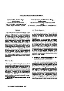
Consider a Timoshenko beam in Figure 1. Denote the displacement of the Timoshenko beam at position i, and time j by w(i, j), and rotation of the Timoshenko beam’s crosssection owing by ϕ(i, j).

φ(i, j+1) = rφ(i+1, j)+(1−2r)φ(i, j)+rφ(i−1, j) (6) Stable solution with the Heat scheme is obtained only if and only if: r = αk/h2 < 1/2 2.6.2

(7)

Scheme for the Flexible Beam Equation

Figure 1. Timoshenko beam

Governing equation of the system is: ρwtt (i, j) = − EIwxxxx (i, j)

+ T wxx (i, j) − cwt (i, j) + f (i, j)

(8)

By modeling this flexible system, we obtain governing, boundary equations, and initial conditions as follows. Governing equations of T-beam is defined as:

4

Minh, Tajwar, Usama, Yeman and Saed

3.1.3

h i ρwtt (i, j) = −K ϕx (i, j) + wxx (i, j) + f (i, j)

Step 3: Apply boundary and initial conditions

(11) Initial conditions approximation from Eq. (19) and noting Eq. (17) and Eq. (18)

h i Iρ ϕtt (i, j) = EIϕxx (i, j) − K ϕ(i, j) + wx (i, j) (12)

w(i, 1) = w(i, 0) = i/2

(21)

ϕ(i, 1) = ϕ(i, 0) = π/6

(22)

Boundary condition approximation from Eq. (14) means for all (i, j) ∈ (0, N ) × [0, ∞), where ρ is uniform mass that the first node is fixed per unit length of the Timoshenko beam. K = kGA is a positive constant that depends on the w(0, j) = ϕ(0, j) = 0 (23) shape of the Timoshenko beam’s cross-section. Iρ is the uniform mass moment while inertia of the Timoshenko In this article, two cases are investigated, comprising beam’s cross-section and EI is bending stiffness of the without control and with PD control. Timoshenko beam. (i) Without control The disturbance d(i, j) and θ(i, j) on the tip payload is generated by: u(j) = 0 (24) d(i, j) = 1 + sin(πij) + sin(2πij) + sin(3πij) (13) θ(i, j) = sin(πij) + sin(2πij) + sin(3πij) τ (j) = 0 (25) Substituting Eq. (24) into Eq. (15) to obtain

Boundary conditions of the system are written as: w(0, j) = ϕ(0, j) = 0 h

M wtt (N, j) − K ϕ(N, j) − wx (N, j)

(14) i

(15)

= u(j) + d(i, j)

Jϕtt (N, j) + EIϕx (N, j) = τ (j) + θ(i, j)

(16)

where w(N, j) is the tip point of the beam. M denotes mass of the payload. J is the inertia of the payload. u(j) and τ (j) are the controllers. Next, the corresponding initial conditions of the beam system are given as w(i, 0) = i/2

(17)

ϕ(i, 0) = π/6

(18)

ϕt (i, 0) = wt (i, 0) = 0

(19)

w(N, j) =2w(N, j − 1) − w(N, j − 2) h i h i 2 2 + k K/M ϕ(N, j − 1) + k /M d(N, j) h 2 − k K/M h w(N, j − 1) i − w(N − 1, j − 1) (26) Substituting Eq. (25) into Eq. (16) to obtain ϕ(N, j) =2ϕ(N, j − 1) − ϕ(N, j − 2) h i 2 − k EI/Jh ϕ(N, j − 1) − ϕ(N − 1, j − 1) h i 2 + k /J θ(N, j) (27)

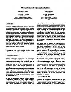
Finally, distributed disturbance along the beam is de- Remark. The graph of Timoshenko beam without control scribed is shown in Figure 2. As we observe, the tip position of h the beam fluctuates around 0, which reflects the bad effect f (i, j) = i/1000L 1 + sin(0.1πij) of external sources or undesired disturbance. However, the (20) i system still keeps its stability. + sin(0.2πij) + sin(0.3πij) (ii) PD control

3.1.2

Step 2: Select Mesh Configuration

Choose T = 10000 and N = 50.

u(j) = −k1 w(N, j) − k1 wt (N, j)

(28)

τ (j) = −k3 ϕ(N, j) − k4 ϕt (N, j)

(29)

5

A Universal Simulation Platform for Flexible Systems

And Eq. (12)

Displacement of string without control

2

w(x,t)(m)

1

0

−1 0 0.2 0.4

100 80

0.6

60 0.8

x(m)

40 1

20 0

ϕ(i, j) =2ϕ(i, j − 1) − ϕ(i, j − 2) h 2 + k EI/Ip h2 ϕ(i + 1, j − 1) − 2ϕ(i, j − 1) i h i 2 + ϕ(i − 1, j − 1) − Kk /Ip ϕ(i, j − 1) h i 2 + k /Ip h w(i, j − 1) − w(i − 1, j − 1) (33)

Time (s)

Figure 2. T beam - without control 303

7

Substituting Eq. (28) into Eq. (15)

Tip position of the beam with PD control

x 10

6

5

y(L,t)(m)

w(N, j) =2w(N, j − 1) − w(N, j − 2) h i h i 2 2 + k K/M ϕ(N, j − 1) + k /M d(N, j) h i 2 − k K/M h w(N, j − 1) h i 2 − k kd/M w(N, j − 1) h i 2 − k kp/M k w(N, j − 1) − w(N, j − 2) i − w(N − 1, j − 1) (30)

4

3

2

1

0

0

20

40

60

80

100

Time(s)

Figure 3. Tbeam - PD control (k1 = k3 = 100 and

k2 = k4 = 30)

Substituting Eq. (29) into Eq. (16) ϕ(N, j) =2ϕ(N, j − 1) − ϕ(N, j − 2) h i 2 − k EI/Jh ϕ(N, j − 1) − ϕ(N − 1, j − 1) h i 2 − k kd/J ϕ(N, j − 1) h i − kkp/J ϕ(N, j − 1) − ϕ(N, j − 2) h i 2 + k /J θ(N, j) (31)

Remark. Unsuitable controllers k1 = k3 = 100 and k2 = k4 = 30, which make the system lose stability, is shown in Figure 3. The shape displacement goes up dramatically without decreasing a trend. Thus, we can conclude that large controllers lead the system to be unstable.

3.1.5

Step 6: Interpretation the result

As we can observe that large controllers k1 = k3 = 100 and k2 = k4 = 30 makes the beam lose its stability, to avoid this Finally, we obtain the approximation for governing equa- problem, we might reduce the magnitude of k2 to 10. tion from Eq. (11) h i 2 Remark. Figure 4 and Figure 5 reflect the beam with PD w(i, j) =w(i, j − 1) − w(i, j − 2) + k /ρ f (i, j) control while we choose suitable controllers k1 = k3 = 100 h i 2 and k2 = k4 = 10. The shape displacement sharply de− k K/ρh ϕ(i, j − 1) − ϕ(i − 1, j − 1) (32) creases from initial condition 1 to about 0. Then, it flutters h 2 + k /ρh2 w(i + 1, j − 1) around this point for a short period before converging as i expected. − 2w(i, j − 1) + w(i − 1, j − 1) 3.1.4

Step 4: Define general equation for each element

6

Minh, Tajwar, Usama, Yeman and Saed

Governing equation of the non-uniform string system is represented by

Displacement of string with PD control

0.6

ρ(i)wtt (i, j) =T (i, j)wxx (i, j) + Tx (i, j)wx (i, j)

w(x,t)(m)

0.4 0.2

+ λx (i)[wx (i, j)]3

0

+ 3λ(i)[wx (i, j)]2 wxx (i, j) + f (i, j) (34)

−0.2 −0.4 0 0.2 0.4

100 80

0.6

60 0.8

x(m)

40 1

20 0

Time (s)

Figure 4. Tbeam - PD control (k1 = k3 = 100 and

k2 = k4 = 10)

for all (i, j) ∈ (0, N )×[0, ∞), where T (i, j) denotes the tension at position x = i, and time t = j. ρ(i) is uniform mass per unit length, which is dependent on the position of the mesh. It can be observed that T and ρ in this case are different from the ones in the above mentioned example, where they are constants. The tension T (i, j) and λ(i) of the string can be expressed as

Tip position of the beam with PD control 0.6

T (i, j) = T0 (i) + λ(i)[wx (i, j)]2

0.5

where T0 (i) = 10(i + 1) and λ(i) = 0.1i. Boundary conditions of the system is given

0.4

y(L,t)(m)

(35)

0.3

w(0, j) = 0

0.2

(36)

0.1

M wtt (N, j) + T (N, j)wx (N, j) + λ(L)[wx (N, j)]3

0

−0.1

0

20

40

60

80

= u(t) + d(t) (37)

100

Time(s)

Figure 5. T beam - PD control (k1 = k3 = 100 and

k2 = k4 = 10)

3.2 Non-uniform String 3.2.1

Step 1: Modeling problem using Hamilton’s method

The corresponding initial conditions of the string system are given as w(i, 0) = i

(38)

wt (i, 0) = 0

(39)

For simulation study, the boundary disturbance d(j) on the tip payload is generated by the following equation

d(j) = 1 + 0.2 sin(0.2j) + 0.3 sin(0.3j) + 0.5 sin(0.5j) (40) Consider a non-uniform string in Figure 6. Denote the disThe time-varying distributed disturbance f (i, j) on the placement of the non-uniform string at position i, and time string is described as j by w(i, j). h i f (i, j) = i × 3 + sin(πij) + sin(2πij) + sin(3πij) (41) 3.2.2

Step 2: Select Mesh Configuration

Choose T = 10000 and N = 50. 3.2.3

Step 3: Apply boundary and initial conditions

Initial conditions approximation from Eq. (39) Figure 6. Non-uniform string

w(i, 0) = w(i, 1)

(42)

7

A Universal Simulation Platform for Flexible Systems

Boundary condition approximation for Eq. (36) w(0, j) = 0

(43)

The approximation for Eq. (37) after substituting Eq. (46)

w(N, j) =2w(N, j − 1) − w(N, j − 2) h i − Kk/M w(N, j − 1) − w(N, j − 2) h i 2 + Kk /M h w(N, j − 1) − w(N − 1, j − 1) h u(j) = 0 (44) − k/h w(N, j − 1) − w(N − 1, j − 1) i The approximation for Eq. (37) when u(j) = 0 − w(N, j − 2) + w(N − 1, j − 1) h i h i 2 2 w(N, j) = 2w(N, j − 1) − w(N, j − 2) − 2k /M sgn(A) + k /M d(j) h i 2 h i3 − k T (N,j)/M h w(N, j − 1) − w(N − 1, j − 1) 2 − λ(N )k /M h3 w(N, j − 1) − w(N − 1, j − 1) h i3 2 h − k λ(N )/M h3 w(N, j − 1) − w(N − 1, j − 1) 2 − 10(L+1)k /M dx w(N, j − 1) h i 2 i + k /M d(j) − w(N − 1, j − 1) (45) (47)

In this article, two cases are simulated, comprising without control and with with exact-model control. (i) Without control

3.2.4 Displacement of non−uniform string without control

Finally, we obtain the governing equation from Eq. (34)

0.6

w(i, j) =2w(i, j − 1) − w(i, j − 2) h 2 + k T (i,j)/ρh2 w(i + 1, j − 1) − 2w(i, j − 1) i 2 0 + w(i − 1, j − 1) + k T (i,j)/ρh h i h i 2 × w(i, j − 1) − w(i − 1, j − 1) − k /ρ f (i, j) h i3 2 0 + k λ (i)/ρh3 w(i, j − 1) − w(i − 1, j − 1) h i2 2 − 3k λ(i)/ρh2 w(i, j − 1) − w(i − 1, j − 1) h × w(i + 1, j − 1) − 2w(i, j − 1)+ i w(i − 1, j − 1) (48)

1.5 1 w(x,t)(m)

Step 4: Define general equation for each element

0.5 0 −0.5 −1 0 0.2 0.4

10 8 6 0.8 x(m)

4 1

2 0

Time (s)

Figure 7. Non-uniform string - without control

(T = 10000)

Remark. Non-uniform string without control are represented in Figure 7. Like above example, the string is still stable, although it undulates around 0 due to undesired external disturbance. (ii) Exact model control u(j) =T0 (L)wx (L, j) − M wxt (L, j) − k1 wt (L, j)− k2 wx (L, j) − sgn [wt (L, j) + wx (L, j)] d¯ (46)

3.2.5

Step 5: Solve for derived or secondary quantities by recursion

Solution is obtained by using Matlab when we use all derived equations from former steps. System parameters and variables are defined in Table 2. Remark. Figure 8 and Figure 9 express the movement of the string with exact control while we choose suitable controller . The shape displacement goes down gradually before converging to stable position, 0, as we expect.

8

Minh, Tajwar, Usama, Yeman and Saed

Displacement of non−uniform string with exact model based control 1

167 x 10 Boundary displacement of non−uniform string without control

0 1

−1 −2

0.6

w(0,t) and w(L,t)(m)

w(x,t)(m)

0.8

0.4 0.2 0 0

−3 −4 −5

0.2 −6

0.4

10 8

0.6

6 0.8

x(m)

−7

4 1

2 0

−8 Time (s)

Figure 8. Non-uniform string - exact model control

0

2

4

6

8

10

Time(s)

Figure 10. Non-uniform string - without control (T = 100)

Boundary displacement of non−uniform string with exact model control

Flexible systems including strings and beams are widely applied in many areas of modern mechanical fields. Ele0.8 mentary structural mechanics is primarily concerned with 0.7 the behavior of line elements, such as rods or beams [19]. 0.6 A beam is an element which carries load between the sup0.5 ports by virtue of its resistance to bending and shearing 0.4 [20]. Defection computations may be used for computing 0.3 the reactions for indeterminate beams and trusses as well as 0.2 the stresses in the members of redundant trusses [21] [22]. 0.1 The current practice of design for a given flexible system 0 0 2 4 6 8 10 is troublesome. Engineers and researchers normally need to use a combination of tools for model building, controller design, and numerical simulation. Additional efforts are necFigure 9. Non-uniform string - exact model control essary to observe the simulation results to check whether the oscillation is damped out at the joints [23], [24]. Thus, a GUI was developed using MATLAB for the simulation of 3.2.6 Step 6: Interpretation the result flexible beam in order to help users to easily use the simuBefore coming out with the appropriate controller as well lation platform [25]. as mesh configurations like above, we tested the string with Capabilities T = 100 and kept the left parameters. (i) Let the user input essential parameters such as approximation nodes , length, time, and controller gains. Remark. We can observe that instability of the string with T = 100 in Figure 10. (ii) Process data using C language and save results under 1

w(0,t) and w(L,t)(m)

0.9

Time(s)

MATLAB data files.

(iii) Read data and plot using MATLAB (3D for Displacement and 2D for Moving) Screenshots and Explanation The main features of this open-architecture platform in It is clear that many scientific & technology problems are Figure 11 include: governed by PDEs and hence this topic became an impor(i) A list of systems which the user can choose from tant and emerging field of research in the recent years. It has to simulate including Euler-Bernoulli beam, Timobeen observed that some of the problems have an analytical shenko beam, exponential beam, string, and nonsolution. PDEs can be classified as elliptic, parabolic or hyuniform string perbolic. The aim is to approximate solutions to differential equations that is to find a function (or some discrete approx(ii) A small window shows a figure, which usually deimation to this function) that satisfies a given relationship scribes a chosen system. between its derivatives on some given region of space and time as well as some boundary conditions along the edges (iii) A group of control buttons: "Choose" button allows of this domain. the user to take a general look at a system to simulate, 4

SimuFlex

9

A Universal Simulation Platform for Flexible Systems

"Run" button runs the program. and "Close" button closes program.

Figure 13. Simulation page - after running

Figure 11. Starting page

Figure 14. Simulation page - clear explanation

Figure 12. Simulation page - before running

(iii) A group of control buttons: "Back" button returns to starting page, "Run" button runs the simulation, "Repeat 1" button replays the with control flexible system and "Repeat 2" button replays the without control flexible system.

The main features of the simulation platform is shown in Figure 12. Several workspaces can be opened and executed 5 Conclusions at the same time. In this article, a deep understanding of flexible systems and (i) A powerful system configuration is provided for easy the way to model and simulate them under external disturconfiguration and viewing of various systems such as bance has been studied. The main contribution of this article is building a general procedure for simulating flexible control gain, N, T, length, and time. systems using finite difference method. In addition, contri(ii) A flexible graphic plotting environment is embedded butions included formulating the general stabilizing condiin the system for easily monitoring and observing the tion for some specific systems with the purpose of verifying control performances. The user can view two working the effectiveness of the presented method. Next, two examenvironments. Firstly, 3D figures help user view the ples are provided to demonstrate the simulating procedure. overall performance of the system and check whether Finally, a Graphical User Interface application, SimuFlex, the designed system is stable or not. And then 2D mov- for flexible systems is introduced. ing figures help user to view the state of the flexible Future works or applications of this proposed work can system over time. be, for example, applying the proposed procedure in a com-

10

Minh, Tajwar, Usama, Yeman and Saed

plete system, represented by partial differential equations [19] D. Johnson, Advanced structural mechanics, vol. 1. Thomas Telford Ltd, 2000. with the purpose of simulation. Furthermore, researchers can find a general stabilizing condition for a system of par- [20] B. Hilson, Basic Structural behavior via Models, vol. 3. Granada Publishing Limited, 1972. tial difference equations.

References [1] A. Smyshlyaev, B. Z. Guo, and M. Krstic, “Arbitrary decay rate for euler-bernoulli beam by backstepping boundary feedback,” IEEE Transactions on Automatic Control, vol. 54, p. 5, 2009. [2] J. Liang, Y. Chen, and B. Z. Guo, “A hybrid symbolicnumerical simulation method for some typical boundary control problems,” Simualtion, vol. 80, p. 11, 2004. [3] S. S. Ge, W. He, B. V. E. How, and Y. S. Choo, “Boundary control of a coupled nonlinear flexible marine riser,” IEEE Transactions on Control Systems Technology, vol. 18, pp. 1080–1091, 2010. [4] R. A. Adomaitis, Y. H. Lin, and H. Y. Chang, “Computational framework for boundary-value problem based simulations,” Simualtion, vol. 74, pp. 28–38, 2000. [5] S. S. Ge, T. H. Lee, G. Zhu, and F. Hong, “Variable structure control of a distributed parameter flexible beam,” Journal of Robotic Systems, vol. 18, pp. 17–27, 2001. [6] I. Karafyllis, P. Christofides, and P. Daoutidis, “Dynamics of a reaction-diffusion system with brusselator kinetics under feedback control,” Physical Review E, vol. 59, p. 372�380, 1999. [7] S. S. Ge, T. H. Lee, G. Zhu, , and F. Hong, “Variable structure control of a distributed parameter flexible beam,” Journal of Robotic Systems, vol. 18, pp. 17–27, 2001. [8] G. Zhu and S. S. Ge, “A quasi-tracking approach for finitetime control of a mass-beam system,” Automatica, vol. 34, pp. 881–888, 1998. [9] S. S. Ge, T. H. Lee, and G. Zhu, “Non-model-based position control of a planar multi-link flexible robot,” Mechanical Systems and Signal Processing, vol. 11, pp. 707–724, 1997. [10] S. S. Ge, T. H. Lee, and Z.Wang, “Model-free regulation of multi-link smart materials robots,” IEEE/ASME Transactions on Mechatronics, vol. 6, pp. 346–351, 2001. [11] E. Camponogara, D. Jia, B. H. Krogh, and S. Talukdar, “Distributed model predictive control,” IEEE Control Systems Magazine, vol. 1, pp. 44–52, 2002. [12] O. Morgul, “Dynamic boundary control of a euler-bernoulli beam,” IEEE Transactions on Automatic Control, vol. 37, pp. 639–642, 1992. [13] M. Fard and S. I. Sagatun, “Exponential stabilization of a transversely vibrating beam by boundary control via lyapunov�s direct method,” Journal of Dynamic Systems, Measurement, and Control, vol. 123, pp. 195–200, 2001. [14] W. F. Inc., “Hamiltonian mechanics,” May 2010. [15] D. Kincaid and W. Cheney, Numerical Analysis. Brooks/Cole Publishing Company, 1991. [16] C. Y. Lam, Applied Numerical Methods for Partial Differential Equations, vol. 2. Prentice Hall, 1994. [17] I. Jacques and C. Judd, Numerical Analysis, vol. 8. Chapman and Hall Ltd, 1989. [18] W. F. Ames, Numerical Methods for Partial Differential Equations, vol. 1. Academic Press, second ed., 1977.

[21] McCORMAC, Structural Analysis, vol. 17. The Haddon Craftsmen Inc, 1960. [22] J. Heyman, Basic structural theory, vol. 3. Cambridge University Press, 2008. [23] F. Ghorbel, J. Y. Hung, and M. W. Spong, “Adaptive control of flexible-joint manipulators,” IEEE Control Systems Magazine, pp. 9–13, 1989. [24] B. de Jager, “Acceleration assisted tracking control,” IEEE Control Systems Magazine, pp. 20–27, 1994. [25] S. S. Ge, T. H. Lee, D. L. Gu, and L. C. Won, “A one-stop solution in robotic control system design,” IEEE Robotics and Automation Magazine, 2000.

Biography Minh Hoang Vu: He is an Erasmus Mundus scholar in Medical Imaging and Applications program. He has a B.Sc. in Control and Automation from National University of Singapore and a M.Sc. in Computer Control and Automation from Nanyang Technological University. His research interests are medical imaging, robotics, and machine vision. Email: [email protected] Tajwar Abrar Aleef: He received his Bachelor of Science in Electrical & Electronic Engineering from American International University-Bangladesh (2016). He is currently enrolled in Erasmus Mundus Joint Master Degree in Medical Imaging and Applications program between University of Burgundy (France), University of Cassino (Italy) and University of Girona (Spain). Email: [email protected] Usama Pervaiz: He is studying in Erasmus+ Joint Master Program in Medical Imaging and Applications; University of Burgundy (France), University of Cassino(Italy) and University of Girona (Spain). He has completed his bachelors in Electrical Engineering with major in signal and image processing from National University of Sciences and Technology, Pakistan. Email: [email protected] Yeman Brhane: He received his BSc. in Electronics and Communication Engineering from University of Mekelle, Ethiopia. He is studying Erasmus Mundus Joint Master Degree in MedicAl Imaging and Applications: University of Buorgogne (France), University of Girona (Spain) and University of Cassino. His research interest includes 3D Image Registration, and Segmentation. Email: [email protected] Saed Khawaldeh: He is an Erasmus Mundus scholar pursuing his masters in Medical Imaging and Applications program:University of Burgundy (France), University of Cassino (Italy) and University of Girona (Spain). He has

A Universal Simulation Platform for Flexible Systems

B.Sc. in Computer and Electronics Engineering from AlBalqa Applied University (Jordan). His research interests are Simultaneous EEG-fMRI Recordings, and Machine Learning. Email: [email protected]

11