A Variable Bin Width Histogram Based Image Clustering Algorithm

2010 2010 IEEE IEEE Fourth International International Conference Conference on Semantic on Semantic Computing Computing

A Variable Bin Width Histogram based Image Clustering Algorithm

Song Gao, Chengcui Zhang, Wei-Bang Chen Department of Computer and Information Sciences The University of Alabama at Birmingham Birmingham, AL, 35294, USA {gaos, zhang, [email protected]} As an extension of traditional clustering, projective clustering is proposed to detect clusters in subspace that corresponds to a subset of dimensions. In [1], a generalized projected cluster is defined as “a set ε of vectors together with a set ∁ of data points such that the points in ∁ are closely clustered in the subspace defined by the vectors ε. The subspace defined by the vectors in ε may have much lower dimensionality than the full dimensional space.” In this paper, we propose a novel projective clustering algorithm by histogram construction to further improve the clustering quality of EPCH (an Efficient Projective Clustering technique by Histogram construction) [2]. The main framework follows from EPCH. The improvement in our algorithm includes: • Histograms are constructed with adaptive binning. For example, the bin width is smaller for dense areas and larger for sparse areas. Since the bin width is not fixed, a dimension tree is constructed to manage the bin width in each image feature dimension. It provides a relatively accurate description of data distribution, while keeping a relatively small number of bins. • The construction of variable bin width histogram is automatic without any user input, i.e., bin width and the number of bins is automatically calculated according to local data distribution. • A new thresholding technique called relative entropy is used to detect dense areas. This technique is robust to the variation of the other factors such as bin number and generates a relatively stable clustering result. The robustness of thresholding between EPCH and that of our proposed algorithm are shown in the experiment section. Another advantage of the new thresholding technique is that it is more interpretable, therefore easier for users to specify. The proposed algorithm consists of five steps: (1) Constructing a variable bin width histogram for each 2dimensional subspace; (2) Detecting dense areas in each 2-d histogram; (3) Converting each data object (e.g., a small image region/segment) into a signature that describes how that data object is projected into different subspaces; (4) Merging similar object signature entries; (5) Assigning data objects to corresponding clusters. In the first step, variable bin width histograms are constructed, with each corresponding to a 2-d subspace. The bin width along each dimension is determined by the

Abstract—In image clustering, digital images can be represented with a large number of visual features corresponding to a high dimensional data space. Traditional clustering algorithms have difficulty in processing image dataset because of the curse of dimensionality. Moreover, similarity between images is measured by the values of partial features. To discover clusters existing in different subspace is known as the projective clustering problem. In this paper, we propose a novel projective clustering algorithm that utilizes dense area detection in variable bin width histograms to form the description of potential cluster candidates. Those candidates with sufficient number of data objects are treated as description of clusters. Relative entropy is used as a density threshold in order to iteratively detect dense areas in each histogram. The construction of variable bin width histogram is automatic. Compared with fixed bin width histogram used in previous projective clustering algorithms, such as EPCH (an Efficient Projective Clustering technique by Histogram construction), variable bin width histogram keeps a nice tradeoff between accurately approximating the underlying distribution and clustering efficiency. Fewer input parameters are required in our proposed algorithm, and the only input parameter required is more robust to variations of other factors such as bin width and is more interpretable to general users. Experiments on an image segmentation dataset show that our algorithm has a better clustering quality than EPCH according to V-Measure. Keywords-image analysis; projective clustering; variable bin width histogram; relative entropy

I.

INTRODUCTION

Clustering represents the process of grouping a set of data objects into classes of similar objects. “Similar” data objects share certain characteristics, such as a value range or a specific value of partial or full correlated feature space. As a method of unsupervised learning, clustering is a statistical technique in image analysis. Moreover, for an image query in multimedia databases, clustering can drastically reduce the query range, thereby improve the system performance. Image segmentation is to assign an ID to each pixel in an image such that pixels with the same ID share certain characteristics, such as color, intensity and texture. Pixels with the same IDs are measured to be similar based on a subset or all of above features. Traditional clustering algorithms have difficulty in processing data objects in high dimensional data space due to the curse of dimensionality. 978-0-7695-4154-9/10 $26.00 © 2010 IEEE DOI 10.1109/ICSC.2010.25

166

underlying data distribution of that dimension. A dimension tree is created to manage each dimension’s bin width information. It is worth mentioning that the user has the option to choose the dimensionality of subspaces for which variable bin width histograms are created. For example, the user can choose to start with 1-d histograms instead of 2-d; however, dense areas on one dimension may hide the existence of noise/outliers in the projection on that dimension. The noises and/or sparse areas can usually be better exposed in a higher dimensional subspace, such as 2-d. The higher the dimensionality of subspaces, the more computing resources needed. As a tradeoff, the default dimensionality of histograms in our framework is 2, and 1-d histogram is used as illustrative examples for easy understanding. Step 2 is an iterative procedure that detects dense areas by applying the proposed relative entropy thresholding in each histogram. Dense areas (a set of bins) are removed from the current histogram, and the threshold is re-calculated until a termination condition is satisfied. In the third step, according to whether data objects drop into one dense area in each histogram or not, a signature (by the definition in [2]) is generated for each data object. A signature represents dense areas in subspaces where the data object is located. In Step 4, those signatures which represent the same or similar subspaces are merged to form one signature which represents that cluster. The merged signatures are then sorted in descending order of their weight which is determined by the size of their corresponding cluster. The higher the weight, the more data objects located in the corresponding subspace. In the end, each data object is associated with one signature with the highest similarity. Data objects having similarity with signatures lower than a threshold are treated as outliers. The top max_no_cluster of signatures are returned as true clusters. Section 2 reviews several representative projective clustering algorithms and explains the main technique used in EPCH. Section 3 describes the motivation of using variable bin width histogram. Section 4 presents the improvement of our clustering algorithm in Steps 1 and 2. Experiment results are shown in Section 5. Section 6 concludes this paper. II.

clustering result is sensitive to the variation of these parameters. EPCH has been shown to give better clustering quality than the above two algorithms. It can detect subspace with arbitrary direction like ORCLUS. Lower dimensional equal bin width histograms are constructed to describe the high dimensional data space. The histogram representation improves the execution performance with certain loss in clustering accuracy as a tradeoff. Different thresholds are automatically driven from the distribution represented in each histogram and used to detect dense bins of each histogram iteratively until a terminating threshold is satisfied, and finally signatures are generated. A signature corresponds to a dense area in a higher dimensional subspace represented by a series of dense areas in a lower dimensional space. Those signatures with a large number of data objects are treated as candidates used to describe projected clusters. Sturges’ rule [4] as shown below is used to generate the bin number k of d-dimensional histogram (e.g., d = 1 or 2). If data does not follow the normal distribution, more bins are preferred. Then k becomes a user input parameter. (1) k = (⌈1+log2N⌉)d In [5, 6], it has been shown that Sturges’ rule does not consider the stochastic nature of a histogram. It works well for sample size N ≈ 100, but leads to an over-smoothed histogram for larger dataset. The threshold of each histogram to detect dense areas is specified to be less than the higher density ρ:

ρ = μ + ( 1 / f − 1)σ

(2)

in which μ is the mean and σ is the standard deviation of the projection distribution. f is the spread of high density areas in the histogram projection, i.e., the desired ratio of dense regions in a histogram It is one of user input parameters. Another main parameter is max_no_cluster, namely the maximum number of clusters the user is interested to uncover. Several disadvantages still exist in EPCH. The clustering result is sensitive to the specification of the f value and the bin number k, and those parameters are difficult for user to estimate. In addition, it is unreasonable to specify the same number of bins for each histogram, which ideally should be determined by the underlying data distribution in that subspace. Finally, the f value is not robust and cannot be easily adapted to different dataset. In other words, one global f value cannot work universally well when the number of bins changes or the distribution of the dataset changes, However, asking a user to guess a reasonable f value for his dataset will be a big burden and challenge, especially given that the impact of f value remains nondeterministic, let alone the computational cost involved in this trial-and-error process. The idea of adaptive bins in histogram is ever proposed in [7] for the case of edge detection. Multidimensional histograms with adaptive bins are used to represent the probability distributions. The bin boundaries are iteratively selected which maximize the Chernoff information. Although this method is not considered in our clustering

BACKGROUND

PROCLUS [3] and ORCLUS [1] are two representatives of projected clustering algorithms. One difference between them is that PROCLUS can detect the interesting subspaces with the spread direction parallel to the original axes, while ORCLUS can detect the interesting subspaces with arbitrary spread direction. However, one common disadvantage of both algorithms is that the number of expected clusters is required as input to the clustering algorithm. Further, PROCLUS requires the user to input the average number of dimensions for the clusters, while ORCLUS needs the user to specify the size of the subspace dimensionality. The

167

algorithm, the experimental comparison will be performed in our future work. III.

where IQR is the sample interquartile range, σ is the sample standard deviation, and n is the number of observations in the sample. Both rules are at the same complexity level as Sturges’ rule, but are well-founded in statistical theory. Since both (3) and (4) can provide a reasonable estimation for bin width, it does not really matter which one to use for this purpose. However, to determine the bin boundaries of sub-regions, using quartile provides a finer partition at the front when compared with that of mean and standard deviation, since the sub-region (interquartile range (IQR)) between the first and the third quartiles covers 50% of data objects while using μ±σ has a larger coverage of approximately 68.27% which may cause a bigger problem of under-partitioning. Therefore, Equation (3) is used in our algorithm to select the bin width of a histogram

MOTIVATION OF USING VARIABLE BIN WIDTH HISTOGRAMS

A. Equal Bin Width and Variable Bin Width Histograms In statistics, a histogram is a graphical illustration of tabulated frequencies, shown as bins. It can be used to plot the density of data. The bins of histogram are generally of the same size (bin width), but not necessarily so. On one hand, a fine setting of bin width gives a good description of underlying distribution of a given dataset. However, it also generates a large number of bins that computationally costly. On the other hand, a rough setting may not reflect the distribution of dataset very well. For example, one bin may combine two or more dense areas, or combine dense areas with sparse areas. Consequently, it may compromise the clustering quality if such histograms are adopted. An advantage of rough setting is that less bins result in exponentially faster processing. Considering the tradeoff between computational cost and accurate description of data distribution, a histogram that combines the advantages of above two types of histograms is preferred for clustering algorithm. Ideally, it should have relatively finer bin width setting on dense areas, but not partition with too many bins on sparse areas. This motivates us to use a variable bin width, variable bin number histogram in our clustering algorithm.

IV.

VARIABLE BIN WIDTH BASED PROJECTIVE CLUSTERING

Assume a D-dimensional dataset contains N data objects. In our case, one data object is a small image region represented by a feature vector of D numerical values that is represented as xi = (xi1, xi2, …, xiD), in which 1 ≤ i ≤ N, and xij (1 ≤ j ≤ D) is the value of the jth feature component of xi. A. Construction of variable bin width histogram A given data range can be divided into three sub-ranges, namely left range, middle range, and right range, by the first quartile q1 and the third quartile q3 of data values in this range. Definition 1: For each dimension (feature) i (1 ≤ i ≤ D), a dimension tree Ti is a binary tree that covers the whole data range, which is derived from the minimum and maximum value of data objects on this dimension. The root node contains the densest area of the current dimension. An inorder traversal visits each sub-range in increasing order of data ranges. Definition 2: A tree node TNij of Ti represents the jth subrange of the whole data range of the dimension i. Some basic information stored in TNij includes: • binNum: the number of bins included in this subrange. • minValue: the minimum value of current sub-range. • maxValue: the maximum value of current sub-range. • ptrLeft: the left pointer that points to the left subrange. • ptrRight: the right pointer that points to the right sub-range. The tree structure can speed up the performance of clustering when it needs to retrieve the bin information of individual sub-areas. The bin width hi,j of node TNij is calculated by (3), in which IQR is the interquartile range of the jth sub-range of dimension i. n is the number of data objects dropping into the jth sub-range of dimension i. Therefore, the number of bins in the current node is calculated as: binNum = range of data / hi,j (5)

B. Histogram Density Estimator and Kernel Density Estimator Kernel density estimation is a non-parametric way of estimating the probability density function of a random variable. Since the kernel with different smoothing parameters is used at each observation, it is smoother as a result compared with histogram density estimator. On one hand, our goal is not to generate an absolute precise estimation for the data distribution, since it is time consuming. The histogram density estimator is converging at faster rate than the kernel density estimator. On the other hand, the selection of the bandwidth of the kernel increases the complexity of the whole operation. Therefore, variable bin width histogram is proposed as a middle ground between kernel density estimation and fixed bin histograms. C. Selection of Bin Width or the Number of Bins The bin width or the number of bins is an important parameter to construct a histogram. As presented in Section 2, Sturges’ rule does not work well for large dataset. Two representatives resulted from more recent studies include Freedman and Diaconis’s rule [8] for bin width selection: h = 2 × IQR × n-1/3 (3) and Scott’s rule [9]: h = 3.5 × σ × n-1/3 (4)

168

In a d-dimensional (0 < d ≤ D) histogram, denote its corresponding subspace as φ and each dimension is φi (i∈ [1,d]). The height of each bin of that histogram is calculated by proportion:

height (binm ) =

right area 13. IF ptrNode->ptrLeft is null Update ptrNode to include the information of the left area 14. IF ptrNode->ptrRight is null Update ptrNode to include the information of the right area 15. Return ptrNode;}

number of objects in binm (6) N × ( hϕ1 ,subϕ ,m × hϕ2 ,subϕ ,m × ... × hϕd ,subϕ ,m ) 1

2

d

where N is the total number of data objects. m is the index of a bin (1≤m≤ total number of bins in the histogram). hϕ ,subm i

Figure 1. Pseudo code for the construction of a dimension tree.

i

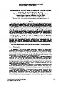
Fig. 2 shows the relationship between sub-areas along one dimension and the corresponding tree node. The vertical axis represents the height of bins.

(i∈[1,d]) represents the bin width of the subφim -th sub-range of the dimension φi. The product (hϕ1 , subϕ ,m × hϕ2 , subϕ ,m × ... × hϕ d , subϕ ,m ) is therefore the 1

2

d

volume of that d-dimensional bin. The pseudo code for constructing a dimension tree on one dimension is shown below: Input: 1. Data array along one dimension: pData[] with length N 2. Start index for current sub-area: st 3. End index for current sub-area: ed 4. Total number of data objects: N Output: 1. Pointer of root node of the dimension tree: ptrNode ptrNode generation_dimension_tree (pData, st, ed, N) { 1. IF the number of data objects in the current area< 0.005*N Return null; /*divide the current data range into 3 sub-ranges: left, middle, and right*/ 2. Calculate the 1st and the 3rd quartiles, namely q1 and q3, of pData ranging from st to ed //generate bin width of the middle area 3. Calculate the bin width mBinWidth of the middle area by (3) 4. Initialize ptrNode to include the information of the middle area 5. IF mBinWidth is 0 Return null; 6. ELSE Calculate the bin number mBinNum of middle area by (5) 7. Use mBinWidth to estimate bin number lBinNum of the left area by (5) 8. Use mBinWidth to estimate bin number rBinNum of the right area by (5) 9. IF lBinNum > mBinNum ptrNode->ptrLeft = generate_dimension_tree (pData, st, q1 , N); 10. ELSE Update ptrNode to include the information of the left area 11. IF rBinNum > mBinNum ptrNode->ptrRight = generate_dimension_tree (pData, q3, ed, N); 12. ELSE Update ptrNode to include the information of the

Figure 2. Mapping between dimension tree nodes and the corresponding sub-ranges along one dimension.

B. Relative Entropy as a Density Threshold Relative entropy [10], also known as the Kullback– Leibler divergence that is a non-symmetric measure of the difference between two probability distributions P and Q has its origin in probability theory and information theory. Usually, P represents the real distribution of data, while Q represents a model or compared distribution of the same data. Definition 3: The relative entropy Hr(X) of a ddimensional histogram is defined as: Hr (X ) =

∑

T i =1

p ( xi ) log 2 ( p( xi ) / q( xi )), X = T

(7)

where X represents the complete set of bins in the current histogram, T is the total number of bins in the current histogram, p(xi) is the normalization of the height of bin i under real distribution, and q(xi) is the normalization of height of the same bin under uniform distribution. p( xi ) =

| xi | /( N × hi ) | xi | / hi = T | xi | T | xi | i =1 h i =1 N × h i i

∑

∑

(8)

where hi = hi1 × hi2 × ... × hid is the volume of the i-th bin in the current d-dimensional histogram.

169

hik , 1≤k≤d, is the bin

previous ones, is added to force the threshold to be updated in that direction. The pseudo code of this procedure is shown in Fig. 3. 1. threshold = calculate the current threshold Hr(X)/T; 2. prevThrd = MAX_VALUE; 3. WHILE (threshold < prevThrd AND Hr(X) ≥ ε) { 4. prevThrd = threshold; 5. find_dense_region (threshold); 6. remove_dense_region (); 7. Update p(xi) and q(xi) of the remaining bins; 8. threshold = calculate relative entropy Hr(X);}

width on the kth dimension, |xi| is the number of objects in bin i. q( xi ) =

where S =

∑

T

N (hi / S ) 1 N × hi 1 S = = T N ( hi / S ) T T i =1 N × h S i

(9)

∑

is the total area that contains data objects

h i =1 i

in the current histogram. From (8) and (9), it can be seen that

∑

T i =1

p( xi ) = 1 ,

∑

simplified as Hr (X ) =

T i =1

q ( xi ) = 1 . Then, Hr(X) can be

Figure 3. Sketch of dense area detection on a histogram.

∑

T i =1

p( xi ) log 2 (T ⋅ p ( xi )), X = T

(10)

In our experiments, ε is usually set to be 0.001. This value is small enough to say safely that current data distribution is sufficiently similar to uniform distribution. As an added advantage, this parameter is also easier to understand for general users, making the specification of input parameter a relatively easier job.

Relative entropy represents the similarity between real distribution of data and uniform distribution of the same data in a d-dimensional subspace. The more similar is a real distribution to a uniform distribution, the more relative entropy approaches 0. Definition 4: The relative entropy hr of a single bin in a d-dimensional histogram is defined as: hr ( x) = p( x) log 2 (T ⋅ p ( x)), x ∈ X (11)

V.

Two versions of our algorithms are implemented in the experiments, namely REH (Relative Entropy on Histogram) and REVBH (Relative Entropy on Variable Bin width Histogram). We compare EPCH with our algorithms in clustering quality on real Image Segmentation data [12]. Image Segmentation dataset is downloaded directly from UCI Machine Learning Repository [12]. To make consistent comparison with EPCH, the original data set is preprocessed as follows: • Some insignificant attributes, namely regioncentroid-col, region-centroid-row, region-pixelcount, short-line-density-5, and short-line-density-2 are removed from feature set. • The feature data is normalized into z-scores, and then each feature (dimension) is linearly scaled into a consistent range, such as [-100, 100], since currently the EPCH requires all feature dimensions having the same data range. Extreme feature values are allowed to remain in the dataset after scaling. V-Measure [11] is used as the measurement of clustering quality in our experiments due to its popularity. All experiments are performed on a PC with Intel(R) Core(TM)2 Duo CPU P8600 2.4GHz, 2GB RAM, and Windows XP SP3.

Usually, an uneven dense area is surrounded by relatively even, sparse areas. If data objects belonging to dense areas are gradually removed from data set, the rest of the data are approaching uniform distribution. Theorem 1: Let all dense bins of a histogram have the same height ph with a relative entropy hr_high and occupy f×T bins (0 ≤ f ≤ 1). Likewise, all sparse areas have the same height pl with a relative entropy hr_low and therefore occupy (1-f)×T of total bins. S is the total area of the corresponding subspace. Then hr_low ≤ (1/T)Hr(X) ≤ hr_high. Proof: hr_high = phlog2(T·ph) and hr_low = pllog2(T·pl). Obviously, hr_high ≥ hr_low.The relative entropy Hr(X) of this histogram is calculated as:

∑ ≥∑ =∑

H r (X ) =

fT fT

T

∑ (T ⋅ p ) + ∑

p h log 2 (T ⋅ p h ) + p l log 2

(1− f )T

(1− f )T

l

EXPERIMENTS

pl log 2 (T ⋅ pl ) p l log 2 (T ⋅ p l )

pl log 2 (T ⋅ pl ) = T ⋅ hr _ low

∴ hr _ low ≤ (1 / T ) H r ( X ) ; Likewise, hr _ high ≥ (1 / T ) H r ( X ) ∴ hr _ low ≤ (1 / T ) H r ( X ) ≤ hr _ high

Relative entropy is used in a greedy algorithm to detect dense bins of a histogram. Adjacent dense bins are combined to form a larger dense area. Then, relative entropy Hr(X), p(xi) and q(xi) of each remaining bins are updated after the removal of dense areas from the current histogram. Input parameter ε is used as a cutoff value for indicating sufficient similarity between the real distribution and uniform distribution in the current subspace. Each time a bin with its hr(x) larger than (1/T)Hr(X) is removed from the current bin set, the updated Hr(X) should be closer to 0 and does so monotonically as shown in line 3 of Fig. 3. The monotonicity awaits final proof. Therefore, another termination condition, i.e., the current threshold (1/T)Hr(X) must be smaller than

Figure 4. Comparison of robustness of threshold parameters.

170

Fig. 4 shows the comparison of robustness to variation of the input threshold parameters between REH and EPCH when different bin width (or different number of bins) is used to construct histograms. In both algorithms, all the subspace histograms have a fixed number of bins (or fixed bin width since data are scaled to the same range) once the parameter is specified by the user. The parenthesized value after each algorithm’s name in Fig. 4 represent the specified threshold parameter value. The two algorithms are tested on different bin numbers, including 12, 20, 30, and 40, among which 12 is calculated according to Sturges' rule, which is a way used in EPCH to generate the number of bins. As can be seen from this figure, for each fixed bin width histogram, our algorithm can generate relatively more stable clustering results under different threshold settings in most cases. There is an exception for REH with threshold value 0.005 when the bin number is set to 12 along each dimension. The larger bin width may cause the occlusion of sparse areas in dense areas and thereby decrease the normalized height of bins. Consequently, all bins may end up with a similar height. Threshold = 0.005 is relatively too high in this case, making the dense area detection terminate too early. In almost all cases, REH has the best clustering quality under different numbers of bins when the threshold is 0.001. In contrast, the clustering quality of EPCH has been significantly affected by the variations in the threshold and the number of bins. EPCH needs to adjust its parameter in order to produce reasonably good clustering result when the number of bins changes. It can be seen from Fig. 4 that when the bin number is 40, the best clustering is achieved by EPCH with a threshold parameter of 4.5 though it is only slightly better than that of REH. However, again it would be too troublesome (and also computationally expensive) for general users to try on so many different combinations of # of bins and threshold values in order to get a reasonable clustering result. The optimal threshold parameters for EPCH, under different numbers of bins (12, 20, 30, and 40), are 3.5, 5.0, 5.0, and 4.5, respectively. As for REH, the optimal threshold under each different number of bins is 0.001 which is also used as the input value for ε in REVBH. The difference between REVBH and the previous two algorithms is that – in REVBH, there is no need to specify the number of bins (or bin width), instead it will be automatically estimated for each data subspace using the method aforementioned. The comparison result in Fig. 5 clearly shows that REVBH has better clustering quality in all cases according to V-Measure. The corresponding data in Fig. 5 is shown in Table I.

TABLE I. V-MEASURE COMPARISON OF OPTIMAL CLUSTERING RESULTS # of Bins 12 20 30 40 Total

REVBH (Th.: 0.001) 0.7265

REH (Th.: 0.001) 0.7012 0.7047 0.6923 0.6735 0.7047

EPCH (Th.) 0.6511 (3.5) 0.6820 (5.0) 0.6210 (5.0) 0.6951 (4.5) 0.6951 (4.5)

VI. CONCLUSIONS In this paper, we propose a new projective image clustering algorithm by using variable bin width histogram. It provides a relatively accurate estimation of data distribution in the projected space while keeping a relatively smaller number of bins compared with fixed bin width histograms. The bin width is calculated automatically according to local data distribution. Because relative entropy has a characteristic that it approaches to zero monotonically in the iterative detection procedure, the threshold for it is relatively easier to specify and understand compared with that of other algorithms, such as EPCH. Experiments show the robustness of our threshold parameter and superior clustering quality of our algorithm in terms of V-Measure. REFERENCES [1]

C. C. Aggarwal and P. S. Yu, “Finding generalized projected clusters in high dimensional spaces,” In Proc. of the 2000 ACM SIGMOD Intl. Conf. on Management of Data, ACM Press, 2000, pp. 70–81. [2] E. K. K. Ng, A. W. C. Fu, and R. C. W.Wong, “Projective clustering by histograms,” IEEE Trans. on Knowledge and Data Engineering, vol. 17, issue 3, pp. 369–383, 2005. [3] C. C. Aggarwal, J. L. Wolf, and P. S. Yu, C. Procopiuc, and J. S. Park, “Fast algorithms for projected clustering,” In Proc. of the 1999 ACM SIGMOD Intl. Conf. on Management of Data, ACM Press, 1999, pp. 61–72. [4] H. A. Sturges, “The choice of a class interval,” Journal of the American Statistical Association, 1926, pp. 65–66. [5] D. W. Scott, “Multivariate Density Estimation: Theory, Practice, and Visualization,” New York: John Wiley & Sons, 1992. [6] D. W. Scott, “Sturges' rule,” WIREs Computational Statistics, vol. 1, 2009, pp. 303–306, doi: 10.1002/wics.035. [7] S. Konishi, A. L. Yuille, J. M. Coughlan, S. C. Zhu, “Statistical Edge Detection: Learning and Evaluating Edge Cues,” IEEE Trans. on Pattern Analysis and Machine Intelligence, vol. 25, issue 1, 2003, pp 57–74. [8] D. Freedman, P. Diaconis, “On the histogram as a density estimator: L2 theory,” Probability Theory and Related Fields, 1981, 57 (4): pp. 453–476. [9] D. W. Scott, “On optimal and data-based histograms,” Biometrika, vol. 66, no. 3, 1979, pp. 605–610. [10] S. Kullback and R. A. Leibler, “On Information and Sufficiency,” Annals of Mathematical Statistics, vol. 22, no. 1, 1951, pp. 79–86. [11] A. Rosenberg and J. Hirschberg, “V-Measure: a conditional entropybased external cluster evaluation measure,” In Proc. of the 2007 Conf. on Empirical Methods in Natural Language Processing, 2007, pp. 410–420. [12] http://archive.ics.uci.edu/ml/datasets/Image+Segmentation

Figure 5. Comparison of optimal clustering quality.

171