Oct 30, 2006 - factorial and fractional factorial designs that are robust against the presence ... for optimal run orders of experimental designs in the presence of ...
A variable-neighbourhood search algorithm for finding optimal run orders in the presence of serial correlation and time trends Jean-Jacques Garroi Peter Goos Departement Wiskunde, Statistiek en Actuari¨ele Wetenschappen Universiteit Antwerpen
Kenneth S¨orensen Centrum voor Industrieel Beleid Katholieke Universiteit Leuven & Departement Milieu, Technologie en Technologiemanagement Universiteit Antwerpen
October 30, 2006 The responses obtained from response surface designs that are run sequentially often exhibit serial correlation or time trends. The order in which the runs of the design are performed then has an impact on the precision of the parameter estimators. This article proposes the use of a variable-neighbourhood search algorithm to compute run orders that guarantee a precise estimation of the effects of the experimental factors. The importance of using good run orders is demonstrated by seeking D-optimal run orders for a central composite design in the presence of an AR(1) autocorrelation pattern. Keywords: AR(1), autocorrelation, central composite design, Doptimality criterion, local search.
1
1 Introduction Response surface designs, such as factorial and fractional factorial designs, central composite designs and Box-Behnken designs, are often run sequentially. Therefore, it is likely that the data exhibit patterns of serial correlation. In that case, the orders in which the runs of the experimental design are carried out has an impact on the precision of the parameter estimates. This article presents a variable-neighbourhood search algorithm for finding efficient run orders for given designs. The problem of finding run orders of standard experimental designs in the presence of serial correlation has received attention from Constantine (1989), who sought efficient run orders of weighing and factorial designs, Cheng and Steinberg (1991), who propose the reverse foldover algorithm to construct highly efficient run orders for two-level factorial designs, Martin et al. (1998b), who presented some results on two-level factorial designs, and Martin et al. (1998a), who discussed the construction of efficient run orders for multi-level factorial designs. Zhou (2001) presented a robust criterion for finding run orders of factorial and fractional factorial designs that are robust against the presence of serial correlation. All these authors concentrated on main-effects and maineffects-plus-interactions models. A problem similar to the one considered in the present article is the quest for optimal run orders of experimental designs in the presence of deterministic time trends. Articles in that area focused on the construction of trend-free or trend-robust run orders, which ensure that the parameter estimates are not impacted by a time trend in the data. For example, Cheng (1990) and Cheng and Steinberg (1991) discussed trend-free run-orders for two-level factorial designs. A different line of research was started by Tack and Vandebroek (2001, 2002, 2003, 2004). Rather than using a given experimental design, they adopted an optimal design approach to select the design and to find an optimal run order simultaneously. As researchers often prefer to work with well-known standard designs, we adopt the same philosophy as Cheng (1990), Cheng and Steinberg (1991) and Martin et al. (1998a,b) and seek run orders for given designs in this article. Although the focus in this article is on the search for optimal run orders in the presence of serial correlation, the presented algorithm is applicable to the problem of finding good run orders of a given design in the presence of time trends too. As the problem of ordering the runs of factorial designs for efficiently estimating first-order models has been studied extensively, we illustrate our algorithm using a popular type of experimental design for estimating secondorder response surface models, namely central composite designs. Constantine (1989), Martin et al. (1998b), Cheng (1990) and Cheng and Steinberg (1991) show that a key feature of run orders for two-level factorial designs that ensure a precise estimation of the factor effects in the presence of serial correlation and time trends is that they require a large number of changes of
2
the levels of the experimental factors. In this paper, we use the newly developed variable-neighbourhood search algorithm to investigate to what extent this result carries over to optimal run orders for central composite designs in the presence of serial correlation. The article is organized as follows. Section 2 provides a description of the statistical model and the design criteria considered in this paper. Section 3 serves as a motivation for this article and illustrates how large the impact of the use of different run orders on the precision of the parameter estimates can be. A variable-neighbourhood search algorithm for seeking efficient run orders is presented in Section 4. Finally, a selection of computational results and a description of the features of the optimal run orders are given in Section 5. A discussion including suggestions for future research concludes the paper.
2 Model and design criteria The algorithm presented in this article is applied to the problem of finding optimal run orders for central composite designs. The model that is usually estimated when this type of experimental design is utilized is the full secondorder model Yt = β0 +
k � i=1
βi xit +
k k−1 � �
βij xit xjt +
i=1 j=i+1
k � i=1
βii x2it + εt ,
where k represents the number of experimental factors, Yt represents the response observed at run t, xit is the level of the ith factor at that run, β0 , β1 , . . . , βkk represent the p = k(k − 1)/2 + 2k + 1 unknown model parameters, and εt is the random error at the tth run of the central composite design. The random errors εt , t = 1, 2, . . . , n with n the number of runs in the design, are assumed to have a zero mean and to follow an AR(1) correlation pattern. If we denote [ 1 x1t . . . x2kt ]� by xt and [β0 β1 . . . βkk ]� by β, the model is given by Yt = x�t β + εt , where εt = ρεt−1 + νt , 0 < ρ < 1, and E(νt ) = 0 and var(νt ) = σν2 for all t. In matrix notation, the model can be written as Y = Xβ + ε, where Y = [ Y1 Y2 . . . Yn ]� , the model matrix X = [ x1 x2 . . . xn ]� and ε = [ ε1 ε2 . . . εn ]� . The covariance matrix of ε and Y is ⎤ ⎡ 1 ρ ρ2 . . . ρn−1 ⎢ ρ 1 ρ . . . ρn−2 ⎥ ⎥ σν2 ⎢ ⎢ ρ2 ρ 1 . . . ρn−3 ⎥ V= ⎥ ⎢ 1 − ρ2 ⎢ .. .. .. .. ⎥ .. ⎣ . . . . . ⎦ n−1 n−2 n−3 ρ ρ ... 1 ρ
3
Under these assumptions, the best linear unbiased estimator is the generalized least squares estimator � −1 ˆ X)−1 X� V−1 Y , β GLS = (X V
(1)
with covariance matrix (X� V−1 X)−1 . Because of computational convenience or ignorance about the presence and nature of the serial correlation, many experimenters however stick to the ordinary least squares estimator � −1 � ˆ XY, β OLS = (X X)
(2)
which has covariance matrix (X� X)−1 X� VX� (X� X)−1 . This led us to consider two different criteria for selecting run orders. First, we seek run orders that maximize |X� V−1 X|1/p . These run orders minimize the volume of the confidence ellipsoid about the unknown model parameters contained in β when the generalized least squares estimator (1) is used. Second, we seek run orders that maximize |X� X(X� VX)−1 X� X|1/p . These run orders minimize the volume of the confidence ellipsoid about the unknown model parameters when the ordinary least squares estimator is applied. The two criteria are D-optimality criteria (Atkinson and Donev (1992), Goos (2002)) which is why the determinants |X� V−1 X|1/p and |X� X(X� VX)−1 X� X|1/p are called Doptimality criterion values and which offers the technical advantage that the coding of the experimental variables does not have an impact on the optimal run order. The optimal run orders depend on the magnitude of the correlation coefficient ρ, but not on the variance σν2 . The quality of a given run order, with model matrix X, is expressed using a Defficiency. For situations in which generalized least squares estimation is used, the D-efficiency of a certain run order with model matrix X is defined as � DGLS =
|X� V−1 X| 1/p , |X�GLS V−1 XGLS |
where XGLS represents the model matrix corresponding to the optimal run order for generalized least squares estimation. For situations in which ordinary least squares estimation is performed, the D-efficiency of a certain run order with model matrix X is defined as 1/p � |X� X(X� VX)−1 X� X| , DOLS = |X�OLS XOLS (X�OLS VXOLS )−1 X�OLS XOLS | where XOLS is the model matrix corresponding to the optimal run order for ordinary least squares estimation. The loss of D-efficiency incurred by not using the optimal run orders is expressed as (1 − DGLS ) × 100% and (1 − DOLS ) × 100% for generalized and ordinary least squares, respectively.
4
3 The impact of the run order Randomization is a keyword in standard textbooks on experimental design. For response-surface designs that are run sequentially, this means that the runs should be carried out in random orders. When the observations are statistically independent, for example when V = σε2 In , each of the run orders leads to the same value, |σε−2 XX|1/p , for the two D-optimality criteria introduced in the previous section. However, in the presence of serial correlation, some run orders lead to substantially smaller values for the D-optimality criterion than others. We illustrate this by means of central composite designs.
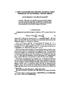
3.1 Central composite designs In general, central composite designs are composed of three types of experimental runs: 1. 2k or, for larger values of k, 2k−f factorial points, 2. 2k axial points at a distance α from the center, and 3. several center points. We denote the number of factorial, axial and center points in the central composite design by nF , nA and nC , respectively. The exact value of α used for the axial points depends on the shape of the experimental region, the number of experimental factors k and technical properties. Common choices for α are √ 1 (when the design region is cuboidal) and 4 nF when the goal is to have a rotatable design for a spherical region. Also the number of center points utilized depends on the number of experimental factors and technicalities such as the potential need for blocking the design (Myers and Montgomery, 1995). A 17-run central composite design for three factors x1 , x2 and x3 is displayed in Table 1. The first eight points in the table are the factorial portion of the design, whereas the points 9-14 are the axial points. The last three points are center runs. A graphical representation of the central composite design is given √ in Figure 1. In this article, we use α = 4 nF for each of the axial runs. The number of possible run orders of a central composite design with nC center runs equals n!/nC ! = (nF + nA + nC )!/nC ! = (2k + 2k + nC )!/nC ! when all factorial points are included in the design. This number increases very rapidly with k, the number of experimental factors. For k as small as two and three center runs, already 6652800 different run orders are possible. For six factors and eight center points, more than 10121 run orders exist. These numbers make it impossible to enumerate all run orders in order to select the best one(s). In the next section, we investigate the range of losses in D-efficiency that can be obtained when random run orders are used for central composite designs with three and six experimental factors.
5
Table 1: Central composite design for three experimental factors. Run 1 2 3 4 5 6 7 8 9 10 11 12 13 14 15 16 17
Label 1 2 3 4 5 6 7 8 9 10 11 12 13 14 15 15 15
x1 −1 −1 −1 −1 +1 +1 +1 +1 −α +α 0 0 0 0 0 0 0
x2 −1 −1 +1 +1 −1 −1 +1 +1 0 0 −α +α 0 0 0 0 0
x3 −1 +1 −1 +1 −1 +1 −1 +1 0 0 0 0 −α +α 0 0 0
+1
x2 +1
x3
-1 -1
x1
+1
-1
Figure 1: Graphical representation of a three-factor central composite design √ with α = 4 nF .
6
40 30 0
10
20
Loss of D−efficiency (%)
40 30 20
Loss of D−efficiency (%)
10 0
0.1
0.2
0.3
0.4
0.5
0.6
0.7
0.8
0.9
0.1
Values of the correlation parameter
0.2
0.3
0.4
0.5
0.6
0.7
0.8
Values of the correlation parameter
(a) 3-factor CCD
(b) 6-factor CCD
Figure 2: Losses in D-efficiency for various values of the correlation parameter ρ when a random run order and generalized least squares estimation are used.
3.2 Random run orders First, we generated 1000 random run orders of a central composite design, involving three center runs, in three factors. Under the asumption that the correlation structure of the residuals is of the AR(1) type, we computed the losses in D-efficiency of each of these run orders with respect to the randomly generated order that produced the largest D-optimality criterion value for generalized least squares estimation. Side-by-side box-plots of the losses in D-efficiency for ρ values between 0.1 and 0.9 obtained in this way are displayed in Figure 2a. The range of the losses clearly increases with ρ, indicating that the impact of the run order on the precision of the estimation is especially important when the serial correlation between the responses is high. However, even for a ρ value as small as 0.1, 5% losses in D-efficiency were observed. For larger correlations, the losses in D-efficiency rapidly become more substantial. We also generated 1000 random run orders for a six-factor central composite design with two center points. Side-by-side box-plots of the losses in D-efficiency for these run orders relative to the best randomly generated order are shown in Figure 2b. It turns out that the losses in D-efficiency are substantially smaller for the six-factor designs than for the three-factor design. For example, the maximum observed losses in D-efficiency were around 2% for a ρ value of 0.1. As can be observed in Figure 2b, the magnitudes of the losses in D-efficiency again increase with ρ. These computational results suggest that using random run orders is generally
7
0.9
not efficient and plead for the use of optimal instead of random run orders. In the next section, we present an algorithmic approach to seeking optimal run orders of given experimental designs.
4 An algorithm for finding optimal run orders Although there is a rich literature on the algorithmic construction of optimal experimental designs (see, for example, Goos (2002)), the problem of finding optimal run orders of standard second-order designs has not received any attention. In this section, we outline the algorithm we propose for that purpose. The algorithm builds on local search algorithms developed for various applications in operational research and operations management.
4.1 Local search algorithms and encoding of solutions In local-search based algorithms for combinatorial optimization, the search for a good solution is done by iteratively making one small change (called a move) to the current solution s. All solutions s� that can be reached in one single move starting from a given solution s are said to be in the neighbourhood of that solution, denoted by N (s). A local optimum is then defined as a solution that does not have any better solution in its neighbourhood, i.e. no improving moves can be made from this solution. Many metaheuristics have been developed, each using a different strategy to escape from these local optima and hopefully reach the global optimum. We define the size of a neighbourhood as the number of solutions it contains, i.e. the number of solutions that can be reached in a single move from the current solution. The size of a neighbourhood usually grows with the size of the problem n. The size n of the problem discussed in this paper is the number of points included in the design. One of the first choices that needs to be made when developing a metaheuristic is the encoding of the solution. Since our problem is to determine the best possible order in which to run a standard experimental design, an obvious choice is to use a permutation encoding. To this end, we assign a rank number to each point in the design and represent a solution as a permutation of these rank numbers. This permutation may contain a repetition of items, if some design points occur more than once. In the design problem discussed in this paper, the center design point is usually repeated nC times, so that the number of unique labels in each permutation equals nF + nA + 1 = n − nC + 1. For example, the 15 labels we utilized for encoding the 17-point three-factor central composite design in Table 1 are shown in the table’s second column. In general, the labels 1, . . . , nF are assigned to the factorial points, the labels nF + 1, . . . , nF + nA are used for the axial points, and the label n − nC + 1 is utilized for all center points in the design. Obviously, many possible “small changes” can be made to any solution. In this context, we should be careful to distinguish between a move type and a move
8
itself. For example, if a solution is represented as a permutation of a set of items, a possible move type is “switch the items in two different positions”. A possible move is “switch the items in positions 1 and 5”. A move type gives rise to a certain neighbourhood structure. Given a move type and a solution, a complete neighbourhood can be derived.
4.2 Variable-neighbourhood search Variable-neighbourhood search (Mladenovi´c and Hansen, 1997) is a recent metaheuristic for combinatorial optimization. As its name suggests, this metaheuristic systematically explores different neighbourhood structures. The main idea underlying variable-neighbourhood search is that a local optimum relative to a certain neighbourhood structure not necessarily is a local optimum relative to another neighbourhood structure. For this reason, escaping from a local optimum can be done by changing the neighbourhood structure. Despite its being a relatively recent development, variable-neighbourhood search has been successfully applied to a wide variety of well-known and lesser-known optimization problems such as vehicle routing (Kytjoki et al., 2005), project scheduling (Fleszar and Hindi, 2004), automatic discovery of theorems (Caporossi and Hansen, 2004), graph coloring (Avanthay et al., 2003) and the synthesis of radar polyphase codes (Mladenovi´c et al., 2003). Usually, variable-neighbourhood search algorithms examine neighbourhoods in a certain order, from small to large. The reason is that small neighbourhoods contain less solutions and can hence be searched in less time than large neighbourhoods. Larger neighbourhoods are only examined when all smaller neighbourhoods have been depleted, i.e. when the current solution is a local optimum of all smaller neighbourhoods. When a solution is found that is a local optimum of all neighbourhoods, a variable-neighbourhood search algorithm uses a perturbation move (called shake in the variable-neighbourhood literature) to jump to a different part of the solution space. The exploration of the different neighbourhoods is then continued from there.
4.3 Neighbourhood structures and perturbation move In our variable-neighbourhood search algorithm1 , we use six different neighbourhoods, half of which have a size that increases proportionally with the size of the problem (i.e. linear neighbourhoods of size O(n)). The other half of the neighbourhoods have sizes that increase according to a second-order polynomial function of the design size (these are quadratic neighbourhoods or neighbourhoods of size O(n2 )). The neighbourhood structures used are summarized in Table 2. The table also contains an instance of each neighbourhood structure 1
It would be more precise to say that our algorithm is a variable neighbourhood descent (VND) method. VND is a deterministic variant of VNS that does not use a random “shaking” move before starting the local search.
9
assuming the current solution s is given by [1,2,3,4,5,5], where label 5 corresponds to a center point. For this example, n thus equals 6 and nC is equal to 2. Table 2: Neighbourhood structures used in the variable-neighbourhood search algorithm. Nk N1
Name Shift right
Size O(n)
N2
Swap adjacent
O(n)
N3
Relabel
O(n)
N4 N5
Swap Move
O(n2 ) O(n2 )
N6
2-Opt
O(n2 )
Description Move all items 1 position to the right, move the last item to position 1, repeat n − 1 times Swap any two items in adjacent positions Use unique labels for all center points, add 1 to each label, change label n + 1 to 1 and labels nF + nA + 2, . . . , n to nF + nA + 1, repeat n − 1 times Swap any two items Move any item to any different position Reverse the solution between any two items
Example [3,4,5,5,1,2]
[1,2,4,3,5,5] [2,3,4,5,5,1]
[1,5,3,4,5,2] [2,3,4,5,1,5] [1,5,4,3,2,5]
To ensure that the number of center points does not change, the relabel move type — contrary to the other move types — requires us to temporarily assign unique labels to all center points. This is done by scanning the permutation from left to right and assigning labels n − nC + 1 to n to the nC center points encountered. For example, starting from solution [1,2,3,4,5,5], we first transform the original encoding into [1,2,3,4,5,6], add 1 to each label and change label 7 to 1, yielding [2,3,4,5,6,1]. The solution is then re-encoded to [2,3,4,5,5,1] by assigning label n − nC + 1 to all points having a label that exceeds this value. The order of the neighbourhoods in our algorithm is such that the larger neighbourhoods are only used when all smaller ones have been exhausted. The order of neighbourhoods of equal size was chosen arbitrarily. In each neighbourhood, we use a steepest ascent move strategy, i.e. we generate all solutions in the neighbourhood, examine their quality and select the best one. This strategy ensures a fast increase of the objective function value. The perturbation scheme we use is very simple: we perform a swap of two randomly selected items twice. This perturbation disturbs the solution enough to prevent the search from immediately converging to the previous local optimum, while maintaining most of the quality of the solution obtained by the previous iteration of the variable-neighbourhood search. A pseudo-code outline of the algorithm is provided in Algorithm 1. In the outline, kmax represents the number of neighbourhoods utilized and k indicates
10
which neighbourhood structure is currently searched by the algorithm. Algorithm 1: VNS algorithm Generate a random initial solution s; repeat Set k ← 1; while k ≤ kmax do Find the best solution s� ∈ Nk (s) ; if s� better than s then Set s ← s� ; Set k ← 1 else Set k ← k + 1 Perturb s; until stopping criterion ;
5 Computational results Using the variable-neighbourhood search algorithm, we have searched optimal arrangements of several central composite designs. The algorithm was coded in R and run on a Pentium 4 2.8 GHz with 1 GB internal memory. To compute the run orders displayed in this section, the algorithm was run for 50 iterations of the main loop (i.e. until 50 perturbations had been performed). Run times were between 5 and 10 minutes for the 17-run central composite design in Table 1. As the best solution was usually found after only a few iterations, the value of 50 was judged to be more than enough. Detailed analysis of the operation of the algorithm shows that all neighbourhoods are indeed used when searching for the optimal solution, even though the linear neighbourhoods are used far more often. The results we display in this section are for the 17-run central composite design in Table 1. The D-optimality criterion values, |X� V−1 X|1/p for generalized least squares and |X� X(X� VX)−1 X� X|1/p for ordinary least squares, of the D-optimal run orders for this design are displayed in Table 3. The beneficial effect of taking into account the correlation pattern when estimating the model is visible through the fact that the D-optimality criterion values are larger for generalized least squares estimation than for ordinary least squares estimation. Even for a design as small as the 17-run central composite design, representing the computational results is difficult as the optimal run orders depend on the correlation parameter ρ and on the estimation method used. Additionally, more than one run order turned out to be D-optimal for any given combination of the correlation parameter and the estimation method. Only a portion of the optimal run orders is displayed here. It is in general difficult to explain how one optimal run order can be transformed into another optimal run order.
11
Table 3: D-optimality criterion values of the D-optimal run orders for ordinary least squares (OLS) and generalized least squares (GLS) estimation. ρ 0.1 0.2 0.3 0.4 0.5 0.6 0.7 0.8 0.9
OLS 200.257262 204.612429 208.257348 210.878225 212.509979 212.256481 208.973890 201.064133 184.908149
GLS 201.269715 208.641952 217.304693 226.979588 237.379511 247.600109 256.385308 261.573121 257.121911
One simple transformation, however, is to reverse the run order of a given optimal design. Another simple possibility is to switch the signs of the values for one or more experimental factors in a given optimal run order. The graphical representations of alternative run orders obtained by switching the signs of the levels of one or more factors would be nothing but mirror images or rotations of the originals.
5.1 Optimal run orders for generalized least squares estimation For generalized least squares estimation, three sets of D-optimal run orders were found. The first set contains run orders that are D-optimal for ρ values between 0 and 0.393. Two run orders from that set are displayed in Figure 3. The second set contains run orders that are D-optimal for ρ values between 0.393 and 0.716. Four run orders from that set are displayed in Figure 4. Finally, the third set contains run orders that are D-optimal for ρ values above 0.716. Two run orders from that set are displayed in Figure 5. An alternative representation of the Doptimal run orders for the generalized least squares estimator is given in Table 4. This representation uses the labels given in the second column of Table 1. Although the run orders displayed in the three figures and Table 4 are substantially different, the first as well as the last run in each of them is a center-point run. Also, sequences of axial runs can be observed in each of the optimal run orders. In these sequences, which can most easily be seen in Table 4, the axial points (which have labels 9 to 14) are arranged so that a given axial point is never preceded or succeeded by its mirror image. Except for large values of ρ, also the factorial points of the central composite design appear in clusters. Within these clusters, the points are arranged so that the values in the columns of the model matrix corresponding to the main effects and two-factor interactions are different in large numbers of pairs of consecutive runs. This result is consistent with the results of Constantine (1989), Cheng and Steinberg (1991) and Martin et al. (1998b) for two-level factorial designs and it is illustrated in
12
14
12
10
4
3
5
7
9
9
5
15
11
1,6,17
13 2
16
12
1,6,17
16 8
8
7
2
3
4
13
14
10
11
15
(a)
(b)
Figure 3: D-optimal run orders for the generalized least squares estimator when 0 < ρ ≤ 0.393.
Table 5 by the model matrix of the D-optimal run order displayed in Figure 3a. The table also contains the Hamming distances, labelled HD, for each consecutive pair of rows of the model matrix. The Hamming distance of a pair of vectors is defined as the number of elements that differ between the two vectors. Within each cluster of factorial points, the Hamming distance between each pair of rows of the model matrix in Table 5 is four. This is the maximum Hamming distance that can be achieved between the rows of any two factorial points in a design involving three factors. Similarly, the Hamming distance between each pair of consecutive rows within the cluster of axial points is always equal to four, which is also the maximum Hamming distance that is possible between any pair of axial points. Table 4: D-optimal run orders for the generalized least squares estimator. The factorial, axial and center points have labels 1 to 8, 9 to 14 and 15, respectively. ρ .0,.393 .393-.716
.716,.999
1 15 15 15 15 15 15 15 15
2 5 3 4 12 13 1 2 5
3 1 8 3 14 10 7 3 1
4 7 2 8 1 4 6 15 15
5 6 4 2 5 3 5 8 6
6 15 9 9 7 2 9 9 13
7 8 1 12 6 8 14 11 12
8 3 5 15 15 15 15 5 14
9 4 6 6 9 7 12 7 9
10 2 7 7 11 5 13 1 8
11 12 13 5 13 1 10 6 2
12 14 11 1 10 6 11 12 4
13 10 9 14 4 12 3 14 3
14 11 14 10 3 9 8 10 10
15 13 12 11 8 14 4 13 11
16 9 10 13 2 11 2 4 7
17 15 15 15 15 15 15 15 15
The arrangement of the axial points and the factorial points in separate clusters however makes that the sum of all Hamming distances between consecutive rows in the model matrix is not at all maximized. We illustrate this by means of the model matrix in Table 5. The maximum Hamming distance between any two consecutive runs of a 17run three-factor central composite design is equal to nine because the column corresponding to the intercept is a column of ones. As a result, the maximum Hamming distance possible is 9 × (17 − 1) = 144. It is clear that this can be
13
16
10
5
16
12
9
4
7
2
13
15
11
1,8,17
14 11
6
7
1,8,17
12 5
3
4
14
15
10
6
13
2
(a)
(b)
16
12
6
16
11
12
2
4
4
15
2
10
1,8,17
3 10
9
3
14
15
1,8,17
11 5
5
7
7
13
14
9
6
3
13
9
(c)
(d)
Figure 4: D-optimal run orders for the generalized least squares estimator when 0.393 ≤ ρ ≤ 0.716.
7
15
2
11
10
11
3
5
16
12
15
6
1,4,17
14 8
6
13
1,4,17
14 2
3
5
8
13
10
9 12
9
16 7
(a)
(b)
Figure 5: D-optimal run orders for the generalized least squares estimator when 0.716 ≤ ρ.
14
Table 5: Model matrix for the D-optimal run order displayed in Figure 3a. The last column of the table contains the Hamming distances between consecutive rows. Run 1 2 3 4 5 6 7 8 9 10 11 12 13 14 15 16 17
I 1 1 1 1 1 1 1 1 1 1 1 1 1 1 1 1 1
x1 0 -1 1 1 -1 0 -1 1 1 -1 0 0 -α 0 0 α 0
x2 0 -1 -1 1 1 0 -1 1 -1 1 0 -α 0 0 α 0 0
x3 0 1 -1 1 -1 0 -1 -1 1 1 -α 0 0 α 0 0 0
x1 x2 0 1 -1 1 -1 0 1 1 -1 -1 0 0 0 0 0 0 0
x1 x3 0 -1 1 1 -1 0 1 -1 -1 1 0 0 0 0 0 0 0
x2 x3 0 -1 -1 1 1 0 1 -1 1 -1 0 0 0 0 0 0 0
x21 0 1 1 1 1 0 1 1 1 1 0 0 α2 0 0 α2 0
x22 0 1 1 1 1 0 1 1 1 1 0 α2 0 0 α2 0 0
x23 0 1 1 1 1 0 1 1 1 1 α2 0 0 α2 0 0 0
HD 9 4 4 4 9 9 4 4 4 9 4 4 4 4 4 2
achieved only when (i) a center point is followed by a factorial point, (ii) a factorial point is followed by a center point, (iii) an axial point is followed by a factorial point (if α �= 1, as it is assumed in this article), or (iv) a factorial point is followed by an axial point (if α �= 1). In the D-optimal run order displayed in Table 5, this happens only four times, namely for runs 2, 6, 7 and 11. For all but one other pair of two consecutive runs, the Hamming distance equals four. Each of these 11 cases corresponds to a sequence of two factorial points or two axial points in the D-optimal run order. Finally, the last pair of runs, an axial point followed by a center point, entails a Hamming distance of two only. This gives a total sum of 82 for the Hamming distances between all consecutive pairs of rows in the D-optimal model matrix in Table 5. In the light of the results of Constantine (1989), Cheng and Steinberg (1991) and Martin et al. (1998a,b), who found that optimal arrangements of factorial designs require large numbers of level changes, it is surprizing that the sum of the Hamming distances in the optimal run order in Table 5 is only 82. It can be shown, however, that designs with a maximum sum of Hamming distances are substantially inferior to the D-optimal run orders. Consider, for example, the run order displayed in Table 6. The model matrix corresponding to this run order has 144 level changes. Nevertheless, its D-efficiency relative to the D-optimal run order in Table 5 is substantially smaller than one. For example, its D-efficiency is only 89.83% when ρ equals 0.3.
15
Table 6: Model matrix for a run order with maximum Hamming distance between each pair of consecutive rows. Run 1 2 3 4 5 6 7 8 9 10 11 12 13 14 15 16 17
I 1 1 1 1 1 1 1 1 1 1 1 1 1 1 1 1 1
x1 0 -1 α 1 0 1 0 -1 0 -1 -α 1 0 1 0 -1 0
x2 0 -1 0 -1 α 1 0 1 0 -1 0 1 -α -1 0 1 0
x3 0 1 0 -1 0 1 α -1 0 -1 0 -1 0 1 -α 1 0
x1 x2 0 1 0 -1 0 1 0 -1 0 1 0 1 0 -1 0 -1 0
x1 x3 0 -1 0 1 0 1 0 -1 0 1 0 -1 0 -1 0 1 0
x2 x3 0 -1 0 -1 0 1 0 1 0 1 0 -1 0 1 0 -1 0
x21 0 1 α2 1 0 1 0 1 0 1 α2 1 0 1 0 1 0
x22 0 1 0 1 α2 1 0 1 0 1 0 1 α2 1 0 1 0
x23 0 1 0 1 0 1 α2 1 0 1 0 1 0 1 α2 1 0
HD 9 9 9 9 9 9 9 9 9 9 9 9 9 9 9 9
5.2 Optimal run orders for ordinary least squares estimation For ordinary least squares estimation, four sets of D-optimal run orders were found. The first set contains run orders that are D-optimal for ρ values between 0 and 0.106. Two run orders from that set are displayed in Figure 6. The second set contains run orders that are D-optimal for ρ values between 0.106 and 0.413. Again, two run orders from that set are displayed in Figure 7. Finally, the third and fourth set contain run orders that are D-optimal for ρ values between 0.413 and 0.711 and above 0.711, respectively. Two run orders from each of these sets are displayed in Figures 8 and 9. Even more consistently than in the optimal run orders for the generalized least squares estimator, sequences of axial and factorial runs can be observed in each of the optimal run orders. The six axial points are clustered in every optimal run order for every ρ value. Again, a given axial point is never preceded or succeeded by its mirror image. The factorial points of the central composite design appear in two clusters of four for any value of ρ. The points in each of these clusters are the same in every D-optimal run order found. When ρ ≤ 0.413, the optimal run orders for the ordinary least squares estimator start and end with a center point, just like all optimal run orders in case the generalized least squares estimator is used. However, for ρ values larger than 0.413, the optimal run orders either start or end with a center run.
16
11
9
5
13
14
15
5
4
2
14
9
10
1,6,17
10 13
7
12
1,6,17
8 3
4
3
7
15
16
16
11
2
8
12
(a)
(b)
Figure 6: D-optimal run orders for the ordinary least squares estimator when 0 < ρ ≤ 0.106.
12
16
3
8
7
9
2
5
5
9
13
15
1,6,17
14 10
11
16
1,6,17
11 4
4
2
12
10
7
8
14
3
15
13
(a)
(b)
Figure 7: D-optimal run orders for the ordinary least squares estimator when 0.106 ≤ ρ ≤ 0.413.
8
7
2
14
14
16
2
3
4
15
7
8
1,6,13
12 15
9
10
1,6,13
9 4
3
5
11
16
17
17
12
5
11
10
(a)
(b)
Figure 8: D-optimal run orders for the ordinary least squares estimator when 0.413 ≤ ρ ≤ 0.711.
17
4
2
17
12
10
9
15
16
16
9
5
7
1,8,13
3 11
6
2
1,8,13
6
15
4
14
14
11
10
12
3
17
7
5
(a)
(b)
Figure 9: D-optimal run orders for the ordinary least squares estimator when 0.711 ≤ ρ < 1.
Table 7: D-optimal run orders for the ordinary least squares estimator. The factorial, axial and center points have labels 1 to 8, 9 to 14 and 15, respectively. ρ .0-.106 .106-.413 .413-.711 .711-.999
1 15 15 15 15 15 15 15 15
2 4 7 8 1 2 1 14 11
3 8 5 2 7 3 6 10 9
4 3 6 3 5 4 5 11 14
5 2 1 4 6 8 7 13 12
6 15 15 15 15 15 15 9 10
7 9 14 1 8 13 11 12 13
18
8 12 10 7 2 11 13 15 15
9 13 11 6 4 9 10 6 4
10 10 13 5 3 14 12 1 8
11 11 9 9 10 12 14 5 3
12 14 12 13 14 11 10 7 2
13 5 2 13 12 9 9 15 15
14 1 4 10 11 1 2 3 5
15 6 3 12 13 5 4 8 1
16 7 8 14 11 6 3 4 6
17 15 15 15 15 7 8 2 7
5.3 Random versus optimal run orders In Section 3.2, it was shown that the order in which a central composite design is run has a substantial impact on the precision of the estimates. This was done by calculating the D-efficiency of each generated random run order with respect to the best random run order found. We can now compute the D-efficiency of each of the random run orders with respect to the D-optimal ones. The resulting side-by-side box-plots are given in Figure 10. The box-plots clearly show that the D-optimal run orders are substantially better than the best of all random run orders that were generated, for all values of the correlation parameter. This demonstrates the usefulness of the variable-neighbourhood search algorithm.
40 30 0
10
20
Loss of D−efficiency (%)
30 20 0
10
Loss of D−efficiency (%)
40
Table 8 contains more detailed information about the losses in D-efficiency when ordinary and generalized least squares estimation are used. For both estimation methods, the table contains 95% confidence intervals for the expected loss in D-efficiency for different values of the correlation parameter ρ. As already indicated in Section 3.2, the losses increase with ρ. Interestingly, random run orders tend to cause larger losses in D-efficiency when ordinary least squares rather than generalized least squares estimation is utilized.
0.1
0.2
0.3
0.4
0.5
0.6
0.7
0.8
0.9
0.1
Values of the correlation parameter
0.2
0.3
0.4
0.5
0.6
0.7
0.8
Values of the correlation parameter
(a) Generalized least squares
(b) Ordinary least squares
Figure 10: Loss of D-efficiency when random instead of D-optimal run orders are used.
5.4 Ordinary versus generalized least squares As practitioners who are unaware of the presence of serial correlation typically use ordinary least squares, it is interesting to compare the optimal run orders
19
0.9
Table 8: 95% confidence intervals for the loss of D-efficiency (expressed in %) when using a random instead of a D-optimal run order for ordinary least squares (OLS) and generalized least squares (GLS) estimation. ρ 0.100 0.200 0.300 0.400 0.500 0.600 0.700 0.800 0.900
GLS 3.458 3.571 6.990 7.207 10.474 10.788 13.802 14.203 16.921 17.402 19.668 20.220 21.963 22.575 23.810 24.472 25.134 25.833
OLS 3.595 3.706 7.555 7.764 11.771 12.064 16.110 16.474 20.609 21.030 24.986 25.449 28.988 29.480 32.393 32.903 34.883 35.404
for the two estimation methods. To this end, we computed the relative Defficiency DOLS/GLS =
� |X�
OLS
XOLS (X�OLS VXOLS )−1 X�OLS XOLS | 1/p |X�GLS V−1 XGLS |
(3)
and the loss in D-efficiency, (1 − DOLS/GLS) × 100%, for different values of ρ. In these expressions, the model matrices XOLS and XGLS contain the optimal run orders for ordinary and generalized least squares estimation, respectively. It turns out that the loss in D-efficiency from using ordinary least squares instead of generalized least squares estimation ranges from 0.50% when ρ = 0.1 to 28.08% when ρ = 0.9. Ordinary least squares estimation is therefore not a good idea for large values of ρ, even not when an optimal run order is used. The optimal run order for ordinary least squares estimation is however quite efficient when the data are analyzed using generalized least squares. This can be verified by evaluating the relative D-efficiency V−1 XOLS | 1/p |X�GLS V−1 XGLS |
� |X�
OLS
and the corresponding loss in D-efficiency. Even for ρ = 0.9, using the optimal run order for ordinary least squares estimation only entails an efficiency loss of 2.896% compared to the optimal run order for generalized least squares. This shows that the D-optimal run orders perform is robust in the sense that they lead to efficient estimates even if a different estimation method is utilized.
5.5 Features of the covariance matrix of the estimators It is well-known that the covariance matrix of the parameter estimator for a central composite design is a sparse matrix when the responses are statistically independent, so that the main effects and two-factor interaction effects can
20
be estimated independently from each other and from the intercept and the quadratic effects. In the presence of an AR(1) correlation pattern, the covariance matrix is no longer sparse, so that most of the parameter estimators are no longer independent. It turns out, however, that the dependence can almost entirely be removed by using D-optimal run orders.
6 Discussion A variable-neighbourhood search algorithm was proposed for finding optimal run orders for given experimental designs. In this article, this was demonstrated assuming an AR(1) autocorrelation pattern and using two versions of the Doptimality criterion and a popular class of second-order response surface design, namely the class of central composite designs. As far as the factorial portion of the central composite designs is concerned, the D-optimal run orders produced by the algorithm exhibit features that are similar to the ones by Constantine (1989), Cheng and Steinberg (1991) and Martin et al. (1998b): the optimal run orders require large Hamming distances between the rows of the model matrix for consecutive factorial runs. The importance of large numbers of changes in values between the elements of the model matrix corresponding to pairs of consecutive factorial points is however in contrast with the overall picture. This is because the clusters of factorial and axial points in the D-optimal run orders limit the Hamming distances between consecutive rows in the full model matrix. Nevertheless, the D-optimal run orders outperform ones which do have a maximum number of level changes. Despite the fact that the number of level changes in the full model matrix is not optimal, there are quite a number of level changes in the columns corresponding to the main effects of the experimental factors. These optimal run orders are therefore especially valuable for experiments involving factors for which it is not too hard, time-consuming or costly to reset the levels independently (for more details about the problem of running experiments in the presence of hard-tochange factors, see, for example Ju and Lucas (2002), Webb et al. (2004), Goos and Vandebroek (2004), Ganju and Lucas (2005) and the references therein). The algorithm presented here will prove a useful tool in the future search for optimal run orders in the presence of serial correlation and time trends. An important aspect of future research in this context will be to adopt a Bayesian perspective. This is because the optimal run orders not only depend on the magnitude of the serial correlation, but also because they depend on the type of serial correlation. In situations where researchers are uncertain about the precise nature of the serial correlation, a Bayesian approach that takes into account a researcher’s prior beliefs will produce compromise run orders that guarantee an efficient estimation of the model parameters whatever the autocorrelation pattern turns out to be. Such a Bayesian approach will also be needed to construct trend-robust run orders when the exact nature of a timetrend is unknown prior to the experiment.
21
Another important aspect of future research is to seek optimal run orders for optimality criteria other than the D-optimality criterion used in this paper. This is especially important for experimental design problems where the focus is on precise prediction rather than on precise estimation of the model. Given the computational complexity of the problem under study, improving the run times for the algorithm is another important concern for future research. One of the most promising research directions in this respect is to seed the algorithm with a high-quality initial solution (instead of a random one, as the current version of the algorithm uses) as this will shorten the time-consuming initial search towards the first high-quality solution. As we have shown in Section 5, good run orders exhibit special structures and it is likely that by carefully studying these, excellent initial solutions can be built.
References A. C. Atkinson and A. N. Donev. Optimum Experimental Designs. Oxford U.K.: Clarendon Press, 1992. C. Avanthay, A. Hertz, and N. Zufferey. A variable neighborhood search for graph coloring. European Journal of Operational Research, 151:379–388, 2003. G. Caporossi and P. Hansen. Variable neighborhood search for extremal graphs. 5. three ways to automate finding conjectures. Discrete Mathematics, 276: 81–94, 2004. C.-S. Cheng. Construction of run orders of factorial designs. In S. Ghosh, editor, Statistical Design and Analysis of Industrial Experiments, pages 423– 439. New York: Marcel Dekker, 1990. C.-S. Cheng and D. M. Steinberg. Trend robust two-level factorial designs. Biometrika, 78:325–336, 1991. G. M. Constantine. Robust designs for serially correlated observations. Biometrika, 76:241–251, 1989. K. Fleszar and K. S. Hindi. Solving the resource-constrained project scheduling problem by a variable neighbourhood search. European Journal of Operational Research, 155:402–413, 2004. J. Ganju and J. M. Lucas. Randomized and random run order experiments. Journal of Statistical Planning and Inference, 133:199–210, 2005. P. Goos. The Optimal Design of Blocked and Split-plot Experiments. New York: Springer, 2002. P. Goos and M. Vandebroek. Outperforming completely randomized designs. Journal of Quality Technology, 36:12–26, 2004.
22
H. L. Ju and J. M. Lucas. Lk factorial experiments with hard-to-change and easy-to-change factors. Journal of Quality Technology, 34:411–421, 2002. J. Kytjoki, T. Nuortio, O. Brysy, and M. Gendreau. An efficient variable neighborhood search heuristic for very large scale vehicle routing problems. Computers and Operations Research, In Press, 2005. R. J. Martin, J. A. Eccleston, and G. Jones. Some results on multi-level factorial designs with dependent observations. Journal of Statistical Planning and Inference, 73:91–111, 1998a. R. J. Martin, G. Jones, and J. A. Eccleston. Some results on two-level factorial designs with dependent observations. Journal of Statistical Planning and Inference, 66:363–384, 1998b. N. Mladenovi´c and P. Hansen. Variable neighbourhood decomposition search. Computers and Operations Research, 24:1097–1100, 1997. ˇ N. Mladenovi´c, J. Petrovi´c, V. Kovaˇcevi´c-Vujˇci´c, and M. Cangalovi´ c. Solving spread spectrum radar polyphase code design problem by tabu search and variable neighbourhood search. European Journal of Operational Research, 151:389–399, 2003. R. H. Myers and D. C. Montgomery. Response Surface Methodology: Process and Product Optimization using Designed Experiments. New York: Wiley, 1995. L. Tack and M. Vandebroek. Trend-resistant and cost-efficient block designs with fixed or random block effects. Journal of Quality Technology, 34:422– 436, 2002. L. Tack and M. Vandebroek. (dt , c)-optimal run orders). Journal of Statistical Planning and Inference, 98:293–310, 2001. L. Tack and M. Vandebroek. Semiparametric exact optimal run orders. Journal of Quality Technology, 35:168–183, 2003. L. Tack and M. Vandebroek. Budget constrained run orders in optimum design. Journal of Statistical Planning and Inference, 124:231–249, 2004. D. Webb, J. M. Lucas, and J. J. Borkowski. Factorial experiments when factor levels are not necessarily reset. Journal of Quality Technology, 36:1–11, 2004. J. Zhou. A robust criterion for experimental designs for serially correlated observations. Technometrics, 43:462–467, 2001.
23