Sep 29, 2007 - CancelAll(N2). Figure 2: Divide-and-conquer algorithm. To find the min-cost flow in N, the algorithm use
A faster algorithm for finding optimal semi-matching Jittat Fakcharoenphol
Bundit Lekhanukit
Danupon Nanongkai
September 29, 2007 Abstract A semi-matching on a bipartite graph G = (U ∪ V, E) is a set of edges M ⊆ E such that each vertex in U is incident to exactly one edge in M . Harvey, Ladner, Lov´ asz, and Tamir consider the matching as an assignment for tasks in U to machines in V . This motivates the definition of the cost of a semi-matching M to be the sum of delay for each task. They give an O(|U ||E|) algorithm based on the Hungarian algorithm for bipartite� matching. In this paper, we give a divide-and-conquer algorithm which runs in time O(|E| |U | log |U |).
1
Introduction
Finding maximum matching in graphs stands out as one of important milestones in combinatorial optimization. This paper considers the problem in bipartite graphs G = (U ∪ V, E), where U is a set of left vertices, V is a set of right vertices. Given G, a matching M is a set of edges, such that each vertex is an end point of at most one edge in M . In many cases, some asymmetry occurs, for example if U is a set of tasks and V is a set of machines, one might want to assign every task a machine. To satisfy this condition, more than one tasks might get assigned to a single machine, i.e., more than one vertex in U is assigned to some vertex in V . Thus, the set of edges corresponding to the assignment in this case is not a matching. Harvey, Ladner, Lov´ asz, and Tamir [1] consider the following relaxation of the maximum bipartite matching problem. A set M ⊆ E is a semi-matching if each vertex u ∈ U is incident with exactly one edge in M . In this case, it is natural to assume that all of the vertices in U have degree at least 1. Semi-matchings has been considered briefly in [2]. In order to define the objective of the problem, Harvey et al. consider the matching as an assignment for tasks to machines. The load-balancing problem in this setting motivates the definition of the cost of a semi-matching M to be the sum of delay for each task. Each task has the same priority; therefore, the total delay for every task assigned to a machine depends only on the number of tasks, i.e., if k tasks is assigned to a machine, the total delay is 1 + 2 + · · · + k. Let degM (v) denote the degree of vertex v in subgraph M . When the matching M is clear from the context, we write deg(v) to mean degM (v). The cost for vertex v ∈ V is degM (v)
costM (v) =
�
i = (degM (v) + 1)(degM (v))/2.
i=1
� The total cost of a semi-matching M is defined to be T (M ) = v∈V costM (v). The problem concerned is to find an optimal semi-matching, a semi-matching with minimum total cost. Harvey et al. show that the optimal semi-matching minimizes simultaneously the makespan, which is the maximum number of tasks assigned to any machine, the flow time, which is an average completion time, and the variance of the loads.
1
Not only that they prove many interesting properties of the optimal semi-matchings, they also show that the problem can be reduced to the min-cost flow problem on graphs with O(|U |+ |V |) nodes and O(|U | + |E|) edges, thus can be solved using min-cost flow algorithms. However, every algorithms for min-cost flow runs in time Ω(mn log n), for graphs with n vertices, and m edges (see [3, 4]). Therefore, they aim for faster algorithms. They give a characterization of the optimal assignment based on cost-reducing paths, and gives two algorithms based on the Hungarian algorithm for bipartite matching and cost-reducing paths. Their algorithms run in time O(|E||U |) and O(min{|U |3/2 , |U ||V |} · |E|).
1.1
Our technique and result
We consider the problem as a special case of the min-cost flow problem. Any semi-matching M can be seen as a flow f . In this context, the optimality condition of Harvey et al. is equivalent to the condition that there is no negative-cost cycle in the residual graph of f . Our algorithm exploits the structure of the graphs and the cost to cancel many negative cycles in a single � of a unit-capacity flow algorithm which runs in time � iteration, using a modification O(|E| |U |). This results in an O(|E| |U | log |U |) algorithm. We note that this is comparable to the running time of the the maximum bipartite matching with an additional logarithmic factor [5, 6, 7, 8]. Our algorithm also works for a slightly general problem. We discuss about this in Section 4.
1.2
Organization
We describe our divide-and-conquer framework and prove its correctness and its running time in Section 2. Informally, the algorithm starts by canceling a set of negative cycles; section 3 discusses this part of the algorithm. Section 4 gives some discussion and generalization. Also, in subsection 4.1, we mention our further result on the case where edges are weighted.
2
The divide-and-conquer framework
Our algorithm is better understood in views of the min-cost flow problem. We start by review the reduction, describe the divide-and-conquer algorithm, and prove the running time. Without loss of generality, we assume that |U | + |V | = O(|E|) as nodes with no adjacent edges can be deleted.
2.1
Optimality characterization revisited
In this section we review the characterization of the optimality of the semi-matching. We describe it in the min-cost flow framework. We start by reviewing how one reduces the problem of semi-matching to the min-cost flow problem. Then, a characterization in a form of augmenting paths is discussed next. We now describe how to reduce the semi-matching problem into a min-cost flow problem with the same optimal cost as in [1]. Given a bipartite graph G = (U ∪ V, E), we construct a directed graph N as follows. Let Δ denotes the maximum degree of the vertices in V . First, add a set of vertices, called cost centers, C = {c1 , c2 , . . . , cΔ } and connect each v ∈ V to ci with edges of capacity 1 and cost i, for all 1 ≤ i ≤ deg(v). Second, add s and t as a source and sink vertex. For each vertex in U , add an edge from s to it with zero cost and unit capacity. For each cost center ci , add an edge to t with zero cost and infinite capacity. Finally, direct each e ∈ E from U to V with capacity 1 and cost 0. The new graph N contains O(n) vertices and O(m) edges. Harvey et al. show that this is a correct reduction,
u1
u2 u3
0,1
0,1
u1 v1 v2
u4
s
0,1
0,1
1,1 0,1
u3
1,1
0,1 0,1
c1 0,∞
2,1
u2
0,1 0,1
v1
2,1
v2
c2
0, ∞
t
0, ∞
3,1
c3
u4
Figure 1: Reduction to the min-cost flow problem. Each edge is labeled with a cost and a capacity constraint. (An example is from [1].) i.e., the cost of the optimal semi-matching in G equals to the cost of the min-cost maximum flow in N . See example in figure 1. Our algorithm based on observation that the largest cost is O(|U |). This allows one to use the cost-scaling framework to solve the problem. For any graph N and flow f in N , let Rf (N ) denote the residual graph of N with respect to f . When N is clear from the context we write Rf to mean Rf (N ). We call any path between two cost centers in Rf an admissible path. An admissible path from ci to cj is reverse if i > j. Note that existence of a reverse admissible path implies the existence of a negative cost cycle. The next lemma states the condition for which a flow f is min-cost. We note that the condition is equivalent to requiring that Rf (N ) has no negative cost cycles. Lemma 1 A flow f is a min-cost flow in N if and only if there is no reverse admissible path in Rf (N ). Proof: Note that f is a min-cost flow if and only if there is no negative cycle in Rf . To prove the “only if” part, assume that there is an reverse augmenting path from ci to cj . We consider the shortest one, i.e., no cost center is contained the path except the first and the last vertices. The edges that effect the cost of this path are only the first and the last ones because only edges incident to cost centers have cost. Cost of the first and the last edge is −i and j respectively. Connecting ci and cj with t results a cycle of cost j − i < 0. For the “if” part, assume that there is a negative-cost cycle in Rf . Consider the shortest cycle which contains only two cost centers, say ci and cj where i > j. This cycle contains an admissible path from ci to cj . Given a max-flow f and a reverse admissible path P , one can find a flow f � with lower cost by augmenting f along P with a unit flow. This is later called path canceling. We are ready to explain our algorithm.
2.2
The algorithm
Our algorithm takes a bipartite graph G = (U ∪ V, E � ) and output an optimal semi-matching. It starts by transforming G into a graph N as described in the previous section. Since the source s and the sink t are always clear from the context, the graph N can be seen as a tripartite graph with vertices U ∪ V ∪ C; later on we denote N = (U ∪ V ∪ C, E). It proceeds by finding an arbitrary max-flow f from s to t in N . This can be done in linear time, because the flow is equivalent to any semi-matching in G.
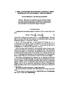
Algorithm CancelAll(N = (U ∪ V ∪ C, E)) 1. If |C| = 1 then halt. 2. Divide C into C1 and C2 . 3. Cancel(N, C2 , C1 ). 4. Divide N into N1 and N2 . 5. CancelAll(N1 ). 6. CancelAll(N2 ). Figure 2: Divide-and-conquer algorithm. To find the min-cost flow in N , the algorithm use a subroutine called CancelAll to cancel all reverse admissible path in f . Lemma 1 ensures that the final flow is optimal. The algorithm is described in Figure 2. The CancelAll works in a divide-and-conquer fashion. Informally, it divides C and solves the problem recursively. It proceeds as follows. Given a set of cost centers C, the algorithm divides C into roughly equal-size subsets C1 and C2 such that, for any ci ∈ C1 and cj ∈ C2 , i < j. This guarantees that there is no reverse admissible path from C1 to C2 . Then it cancels all reverse admissible paths from C2 to C1 . To cancel the rest of the reverse admissible paths, it does so recursively. It divides the problems into N1 and N2 , whose cost centers are C1 and C2 respectively. The division process is described later in this section. It then solves N1 and N2 . In section 3�we describe algorithm Cancel that cancels all admissible paths from C2 to C1 in time O(|E| |U |). After this step, we need to cancel all reverse admissible paths between cost centers “inside” each Ci . The rest of this section is devoted to describing how one gets the subproblems and the correctness of the algorithm. We first describe how to find N1 and N2 . After step 3 in algorithm CancelAll, let S be a set of vertices in N which is reachable from C2 . S can be constructed in O(|E|) time using any linear-time graph searching algorithm. Let N2 be a subgraph of N induced by S and N1 be a subgraph induced by the rest of the vertices. The following two lemmas proves the correctness. Lemma 2 Assume that there is no reverse admissible paths from vertices in C2 to vertices in C1 . Let S be a set of vertices reachable from C2 . Any admissible path between two cost centers in C1 does not intersect S. Proof: Assume, for the contradiction proof, that there exists an admissible path from x to y, where x, y ∈ C1 , that contains a vertex s ∈ S. Since s is reachable from some vertex z ∈ C2 , there must exists an admissible path from some vertex in z to y; this leads to a contradiction. Lemma 3 CancelAll(N ) cancels all reverse admissible path in N . Proof: All reverse admissible paths from C2 to C1 are cancelled in Step 3. Then, Lemma 2 implies that in our dividing step, all reverse admissible paths between pairs of cost centers in C1 remains entirely in N1 . Furthermore, vertices in any reverse admissible paths between pairs of cost centers in C2 must be reachable from C2 ; thus, they must be inside S. Therefore,
after the recursive calls, no reverse admissible paths between pairs of cost centers in the same subproblems Ci are left. The lemma follows if we can show that in these processes we do not introduce more reverse admissible paths from C2 to C1 . To see this, note that all edges between N1 and N2 remains untouched in the recursive calls. Moreover, these edges are directed from N1 to N2 , because of the maximality of S. Therefore there is no admissible path from C2 to C1 .
2.3
Analysis of the running time
We analyze the running time for CancelAll as it dominates the running time of the algorithm. Let T (n, n� , m, k) denote the running time of the algorithm when |U | = n, |V | = n� , |E| = m, and |C| = k. For simplicity, assume that k is a power of two. In Section 3, we show that Cancel � runs in time O(|E| |U |). With that assumption, we can write the running time recurrence as √ T (n, n� , m, k) ≤ c · m n + T (n1 , n�1 , m1 , k/2) + T (n2 , n�2 , m2 , k/2), for some constant c, where ni , n�i , and mi denote the number of vertices and edges in Ni , respectively. We recall that each edge participates in at most one of the subproblems; thus, m1 + m2 ≤ m. √ To see that this recurrence solves to T (n, n� , m, k) = O(m log k n), assume that T (n, n� , m, k) ≤ √ c� · m n · log k for some c� . Plugging into the above recurrence, we have √ T (n, n� , m, k) ≤ c · m n + T (n1 , n�1 , m1 , k/2) + T (n2 , n�2 , m2 , k/2), √ √ √ ≤ c · m n + c� · m1 n1 · log(k/2) + c� · m2 n1 · log(k/2) √ √ ≤ c · m n + c� · m n · log(k/2) √ √ √ = c · m n + c� · m n · log k − c� · m n √ = c� · m n log k, if c� ≥ c. Since k = O(|U |), we have the main result. Theorem 1 (Main theorem) � Given a bipartite graph G = (U ∪ V, E). An optimal semimatching can be found in O(|E| |U | log |U |) time.
3
Canceling paths from C2 to C1
In this section we describe an algorithm that cancels all admissible paths from C2 to C1 in Rf , which can be done by finding max flow from C2 to C1 . To simplify the presentation, we assume that there is a super-source s and super-sink t connecting to vertices in C2 and in C1 , respectively. First we note that N is unit capacity. Thus, any unit-capcity max-flow algorithm can be used in this step. The best known algorithm for this case, e.g., an O(min{n2/3 , m1/2 }m) algorithm by Even-Tarjan [9] and Karzanov [6]. However, we can expliot the structure of the problem � and show that the algorithm based on Dinic’s blocking flow algorithm [10] runs in time O(|E| |U |). We give an outline of Dinic’s blocking flow algorithm. Given a network R with source s and sink t, a flow g is a blocking flow in R if every path from the source to the sink contains a saturated edge, an edge with zero residual capacity. A blocking flow is usually called a greedy flow, since the flow cannot be increased without any rerouting of the previous flow paths. In a unit capacity network, depth-first search can be used to find blocking flow in linear time.
Dinic’s algorithm works in layer graphs. A layer graph is a subgraph whose edges are in at least one shortest path from s to t. This condition implies that we only augment along the shortest paths. The algorithm proceeds by successively find blocking flows in the layer graphs of the residual graph of the previous round. The following is an important property (see [3, 4, 11], for proofs). It states that the distance between the source and the sink always increases after each blocking flow step. Lemma 4 Let di be a length of the shortest s − t path in residual graph at the ith iteration. di+1 > di for all valid i. The lemma can be used to show that Dinic’s algorithm terminates after n rounds of the blocking flow step, where n is the number of vertices. Since after the n-th round, the distance between the source is more than n, which means that there is no augmenting path from s to t in the residual graph. The number of rounds can be improved for certain classes of problems. Even and Tarjan [9] and Karzanov [6] show that in unit capacity networks, Dinic’s algorithm terminates after min(n2/3 , m1/2 ) rounds, where m is the number of edges. Also, in unit networks, √ where every vertex has in-degree one or out-degree one, Dinic’s algorithm terminates in O( n) time (see, e.g., Tarjan’s book [11]). Since the network we use is very similar to unit networks, we are able to show that Dinic’s √ algorithm also terminates in O( n) in our case. For any flow f , a residual flow f � is a flow in a residual graph Rf of f . If f � is maximum in Rf , f + f � is maximum in the original graph. The following lemma relates the amount of the maximum residual flow with the shortest distance from s to t in our case. The proof is a modification of Theorem 8.8 in [11]. Lemma 5 If the shortest s − t distance in the residual graph is d > 4, the amount of maximum residual flow is at most O(|U |/d). Proof: A maximum residual flow in a unit capacity network can be decomposed into a set P of edge-disjoint paths where the number of paths equals to the flow value. Each of these paths are of length at least d. Clearly, each path contains the source, the sink, and exactly two cost centers. Now consider any path P ∈ P of length l. It contains l − 3 vertices from U ∪ V . Since the original graph is a bipartite graph, at least �(l − 3)/2 ≥ �(d − 3)/2 ≥ (d − 4)/2 vertices are from U . Note that each path in P contains a disjoint set of vertices in U , since a vertex in U has in-degree one. Therefore, we conclude that there are at most 2|U |/(d − 4) paths in P. The lemma follows since each path has one unit of flows. From these two lemma, we have the main lemma for this section. � Lemma 6 Cancel terminates in O(|E| |U |) time. Proof: Since each�iteration can be done in O(|E|) time, it is enough to prove that the algorithm The previous lemma implies that the amount of maximum terminates in O( |U | rounds. � � residual flow after the O( |U |)-th rounds is O( |U |) units. The lemma thus follows because after that the algorithm augments at least one unit of flow for each round.
4
Discussion and generalizations
The problem can be viewed in a slightly more general version. In Harvey et al., the cost functions for each vertex v ∈ V are the same. We relax this condition, allowing different function for each
vertex. More precisely, for each v ∈ V , let fv : Z+ → R be a non-decreasing function. The cost for matching M on vertex v is fv (degM (v)). In this general cost, the transformation similar to what described in Section 2.1 can still be done. While the size of set C of cost centers might not be |U |, it is O(|E|),� because it is the numbers � of different values of fv . Therefore, our algorithm runs in time O(|E| |U | log |C|) = O(|E| |U | log |E|).
4.1
Weighted case
The problem can be generalized to the weighted case as follows. In this case, each task u when assigning to machine v has an associated weight wuv , which is the cost incurred for unit delay. Each task still requires unit processing time. Note that one can show that the case where each task has unit processing cost but different delay can be reduced to this case as well. After assigning tasks to machine, the cost of the assignment is the sum of the products of the delay and the weight of the tasks. We note that, unlike the previous case, the cost depends also on the order in which the tasks get processed in each machine. However, given a set of tasks assigned to any given machine, one can verify that the best ordering is one where the larger weight tasks get processed before the smaller ones. Therefore, we define the cost of the weighted semi-matching accordingly. Again, let degM (v) denote the degree of v in the semi-matching M . Consider a list of nodes u1 , u2 , . . . , udegM (v) matched with v, ordered according to their weights �deg (v) with node v is thus costM (v) = i=1M i · wui v . Finally, wui v decending. The cost associated� the cost of the semi-matching M is v∈V costM (v). In [12], we show that the weighted version can also be reduced to the min-cost max-flow problem in a network with |U ||E| edges. We also describe an O(|U ||E| log |U |)-time algorithm for this weighted case. The algorithm is essentially a successive shortest path algorithm with a special data structure to improve the running time of Dijkstra’s algorithm.
References [1] N. J. A. Harvey, R. E. Ladner, L. Lov´ asz, T. Tamir, Semi-matchings for bipartite graphs and load balancing, J. Algorithms 59 (1) (2006) 53–78. [2] E. Lawler, Combinatorial Optimization: Networks and Matriods, Dover, 2001. [3] R. K. Ahuja, T. L. Magnanti, J. B. Orlin, Network flows: theory, algorithms, and applications, Prentice-Hall, Inc., 1993. [4] A. Schrijver, Combinatorial optimization : polyhedra and efficiency, volume A, paths, flows, matchings, chapter 1-38, Springer, 2003. [5] T. Feder, R. Motwani, Clique partitions, graph compression and speeding-up algorithms, J. Comput. Syst. Sci. 51 (2) (1995) 261–272. [6] A. Karzanov, On finding maximum flows in networks with special structure and some applications, Matematicheskie Voprosy Upravleniya Proizvodstvom 5 (1973) 81–94. [7] J. Hopcroft, R. Karp, An n5/2 algorithm for matchings in bipartite graphs, SIAM J. on Computing 2 (1973) 135–158. [8] A. Goldberg, R. Kennedy, An efficient cost scaling algorithm for the assignment problem, Mathematical Programming 71 (1995) 153–177.
[9] S. Even, R. E. Tarjan, Network flow and testing graph connectivity, SIAM J. Comput. 4 (4) (1975) 507–518. [10] E. A. Dinic, Algorithm for solution of a problem of maximum flow in networks with power estimation, Soviet Mathematics Doklady 11 (1970) 1277–1280. [11] R. E. Tarjan, Data structures and network algorithms, Society for Industrial and Applied Mathematics, 1983. [12] J. Fakcharoenphol, B. Lekhanukit, D. Nanongkai, An algorithm for weighted semimatching, manuscript (2005).