A Variable Selection Procedure for X-ray Diffraction

A Variable Selection Procedure for X-ray Diffraction Phase Analysis DAEWON LEE, HYESEON LEE, CHI-HYUCK JUN,* and CHANG HWAN CHANG Department of Industrial and Management Engineering, POSTECH, Pohang 790-784, Korea (D.L., H.L., C.-H.J.); and Characterization & Analysis Department, Research Institute of Industrial Science & Technology, Pohang 790-600, Korea (C.H.C.)

The X-ray diffraction method has been widely used for qualitative and quantitative phase abundance analysis of crystalline materials. We propose the use of partial least squares when building the calibration model for a quantitative phase analysis based on X-ray diffraction spectra. We also propose a variable selection procedure to reduce the measurement points in terms of angles as an alternative to using the whole pattern. The proposed method is based on the variable importance in projection derived from the partial least squares and it considers some practical issues regarding the angle measurement. The method was particularly applied to the simultaneous determination of weight fractions of some iron oxides. It was found that the number of measurement points can be reduced to 30 percent of the total number of points with a small sacrifice in prediction error. Index Headings: Calibration; Desirability function; Phase analysis; Partial least squares; PLS: Variable selection; X-ray diffraction; XRD.

INTRODUCTION Because every crystalline material gives a unique X-ray powder diffraction (XRD) pattern independent of other materials, with the intensity of each pattern proportional to that material’s concentration in a mixture, the X-ray diffraction method has been widely used for qualitative and quantitative phase analysis of powder mixtures. The quantitative phase analysis by X-ray powder diffraction is based on using the relative intensity of major peaks of each phase in the mixture sample or even the full diffraction pattern.1–3 For the rapid determination of concentrations of one or more chemical components based on spectra data, some statistical methods have been used in the area of chemometrics.4 Particularly, partial least squares (PLS) regression is popularly employed when building a calibration model because it is effectively applied even if there is a high multicollinearity among spectrum intensity values (or variables) and if there is a much larger number of variables than there are samples.5–7 Many other tools are introduced in the work of Luo8 that can be applied to X-ray spectrometry. Partial least squares has often been applied to X-ray fluorescence spectrometry.9,10 However, there has been little study on statistical analysis applied to Xray diffraction spectra. To our knowledge, the use of partial least squares on X-ray diffraction spectra is limited to the works of Artursson et al.11 and Karstang et al.,12 where they mainly studied data preprocessing methods to enhance modeling performance. When building a calibration model, we may use the whole X-ray diffraction pattern if it is available. For the rapid determination of concentration of a component of interest in a real process, however, the use of the whole pattern may not be Received 12 March 2007; accepted 12 September 2007. * Author to whom correspondence should be sent. E-mail: chjun@ postech.ac.kr.

1398

Volume 61, Number 12, 2007

efficient because the measurement time increases as the number of measurement points increases. This indicates the need for variable selection to reduce the measurement time, with a small sacrifice in the prediction power of the calibration model. In other words, a procedure must be established for selecting variables when building a calibration model in order to measure only the selected variables in a real on-line process. A number of methods have been available for the variable selection. Chong and Jun13 demonstrated from a simulation study that the use of the variable importance in projection (VIP) index under the partial least squares regression performed well even when a high multicollinearity is present among variables. Some other studies are available in regard to the variable selection methods applied to spectroscopy data.14,15 In the present study, a statistical approach to the quantitative phase analysis is proposed for the determination of one or several concentrations simultaneously, based on the partial least squares regression. A variable selection procedure based on the variable importance in projection is also proposed for reducing the number of measurement points in a diffraction pattern. The proposed procedure was particularly applied to the simultaneous determination of weight fractions of two iron oxides. Its performance was evaluated according to various cutoff values involved and compared with the stepwise method. Particularly, when optimizing the parameters of the proposed procedure, the desirability function approach was employed by considering the tradeoff between angle measurement effort and calibration model performance.

EXPERIMENTAL Measurement of the X-ray Diffraction Pattern. A total of 75 iron ore samples containing different concentrations of iron and iron oxides such as FeO and Fe2O3 were obtained in a pilot plant using Hammersley fines ore mixed with CaCO3 as the subsidiary raw material. These samples were taken randomly because any type of experimental design is not possible. Typical chemical analyses are Fetotal ¼ 67.4;77.8%; FeO ¼ 10.0;26.5%; CaCO3 ¼ 11%; SiO2 ¼ 0.5;1.4%; and Al2O3 ¼ 0.2;0.3%. The wet chemical analysis is certainly a reliable and sensitive method for determining the amount of iron and iron oxides and was used as a reference method for the XRD analysis. The standard error of the wet chemical analysis of iron ore was calculated to be 0.5%, 0.6%, and 0.4% for metallic iron, FeO, and Fe2O3, respectively. The total iron (Fetotal) and FeO were determined by the wet chemical analysis using the standard methods of KS E 3013 and KS B 3016, respectively.16,17 The metallic iron (Femetal) was determined by titration with potassium dichromate. Fe2O3 was calculated by using Fe2O3 (%) ¼ 0.699[Fetotal(%)  Femetal(%)  0.777 FeO(%)]. The X-ray powder diffraction pattern is the intensity

0003-7028/07/6112-1398$2.00/0 Ó 2007 Society for Applied Spectroscopy

APPLIED SPECTROSCOPY

employed, then the dimensions of T, P, U, and Q will be (n 3 A), (p 3 A), (n 3 A), and (m 3 A), respectively. The variable importance in projection (VIP) index has been proposed as a measure of importance of each variable contributing the response of interest.13 After PLS is performed, the VIP for the jth variable is obtained by vffiffiffiffiffiffiffiffiffiffiffiffiffiffiffiffiffiffiffiffiffiffiffiffiffiffiffiffiffiffiffiffiffiffiffiffiffiffiffiffiffiffiffiffiffiffiffiffiffiffi u A A u X X VIPj ¼ tp ð2Þ w2ja b2a tTa ta = b2a tTa ta a¼1

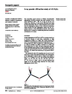
FIG. 1. Measurement of X-ray diffraction pattern.

spectrum as a function of the 2h angle, as shown in Fig. 1. The XRD patterns of the samples were recorded using a Rigaku D/ MAX 2500V diffractometer operating at 50 kV and 180 mA in ˚ ) and a rotating anode type. Cu Ka radiation (k ¼ 1.5405 A graphite monochromator for diffracted beam were used. A continuous scanning mode was adopted with a scanning speed of 58(2h)/min. The XRD patterns over an angular range of approximately 258 to 858 in 2h were collected, and the whole scanning time for each XRD pattern was 12 min and the sampling time was 2 to 10 s. Partial Least Squares and Variable Selection. Partial least squares is known to be most suitable for spectrum-type data having high multicollinearity among variables. Suppose that the intensity values of the XRD pattern are measured at each of p variables (2h angles) on each of n samples and that the actual weight fractions of m phases are measured on each sample. Let X be the (n 3 p) data matrix and let Y be the (n 3 m) response matrix of m response (or phase) variables. Then, the PLS model can be expressed as follows: X ¼ TPT þ E

ð1aÞ

Y ¼ UQT þ F

ð1bÞ

and ua ¼ ba ta þ h;

a ¼ 1; . . . ; A

ð1cÞ

where ta and ua are the ath latent vectors of X and Y, respectively, and T and U are the corresponding score matrices. P and Q are called as loading matrices of X and Y, respectively. Also, ba is the regression coefficient between two score vectors. These quantities can be estimated through the nonlinear iterative partial least squares5,18 (NIPALS) algorithm. In Eq. 1, E and F represent random error matrices of X and Y, respectively, whereas h is a random error vector in the regression model. Verbally, PLS searches for a set of latent vectors that performs a simultaneous decomposition of X and Y under the constraint that these latent variables explain as much as possible of the covariance between X and Y. When we predict the response variables, the number of latent variables is an important factor for quantification accuracy. The number of latent variables is usually chosen by a cross-validation considering the proportion of variations explained by each latent variable. If A denotes the number of latent variables

a¼1

where wja is a weight on the jth variable in the ath latent variable, which is derived from the NIPALS algorithm. Because the average of the squared VIP over all variables is 1, the ‘‘greater than one’’ rule is generally used as a criterion for selecting significant variables. Suppose that a set of training and test data are given, where the input spectra are XRD patterns and the response variables are their weight fractions measured by wet chemical analysis. The calibration model was constructed only with the training data and the test data was used for evaluating the model performance. When building our calibration model, the number of latent variables was chosen by leave-one-out crossvalidation, which is typically used in chemometrics. As an accuracy measure for the kth response variable of a model, the mean absolute deviation (MAD) was used, which is determined as follows: MADk ¼

nT 1 X jyik  yˆ ik j nT i¼1

ð3Þ

where nT is the number of samples in a training data set or test data set and yˆ ik is the predicted kth response of the ith sample. Although the mean squared errors criterion is generally more popularly used, the MAD criterion was adopted here because its size can be directly compared with individual data (it has same unit as the response variable) and it may be less sensitive to a few large errors. In order to determine suitable ranges of angles for obtaining an XRD spectrum, the following variable selection procedure is proposed. Although angles are discrete, several ranges of consecutive angles may be desirable for experimental purposes. Too many intermittent intervals containing small points of angles may not be recommended for an efficient measurement. The proposed variable selection method is as follows: Step 1. Select angles whose VIPs are greater than a specified threshold v. When the selected angles appear consecutively, group them as an interval. Step 2. If two adjacent intervals are within d1, then merge the two intervals into one. As a result, all angles belonging to two intervals will be selected. Step 3. If an interval has a length smaller than d2, then delete the interval. The above procedure has three parameters to be determined. As stated earlier, a value close to 1.0 is recommended for the VIP threshold v. More angles will be selected if a lower value is chosen, whereas fewer angles will be selected if a higher value is chosen. At the extreme, all angles will be selected by choosing v ¼ 0 regardless of d1 and d2. Obviously, a calibration model having a larger number of angles may lead to a smaller prediction error. There is a tradeoff between angle measurement effort and model performance. Therefore, the value of v

APPLIED SPECTROSCOPY

1399

should be selected by considering this tradeoff. The values of d1 and d2 can be determined through a cross-validation. A larger value of d1 may lead to a smaller number of intermittent intervals covering larger points of angles. Meanwhile, a larger value of d2 results in a smaller number of intervals, as well as a smaller number of angles. The finally selected intervals are recommended for use when gathering new data and predicting concentrations of chemical components. To validate the above procedure more objectively, we will report the results by comparing the ones from other possible methods. The PLS model was reconstructed using the selected intervals, where the number of latent variables was determined by the leave-one-out cross-validation method. Parameter Selection By Desirability Approach. In order to build a more accurate calibration model with a smaller number of measurement points, we need to find the best combination of parameters (v, d1, d2). However, there is a tradeoff between angle measurement effort and model performance. To this end, we employed the desirability function approach developed by Derringer and Suich,19 which involves simultaneous consideration of multiple response characteristics. In our problem, we consider three response variables, that is, the percentage of selected measurement points (q1), MAD for FeO (q2), and MAD for Fe2O3 (q3), which are controlled by (v, d1, d2). Here, q2 and q3 are validation MADs obtained from leave-one-out cross-validation on training data. These three responses are of ‘‘The-SmallerThe-Better’’ type. The desirability of each response takes a value between 0 (least desirable) and 1 (most desirable). The desirability function in our case was defined as follows: q1 is most desirable at 0 and least desirable at 100 (%), whereas q2 and q3 are most desirable at 0 but least desirable at 2. It was also assumed that the desirability function of each response is linear. These desirability functions are shown in Fig. 2a. The overall desirability D is calculated by combining individual desirability using the following geometric mean with weights:20 D ¼ ð f1a1 f2a2 f3a3 Þ1=ða1 þa2 þa3 Þ

ð4Þ

where fj and aj are the desirability function and the relative weight of the jth response, respectively. We can easily select the best set of (v, d1, d2) with maximum D among the candidate combinations as shown in Fig. 2b.

RESULTS AND DISCUSSION As mentioned in the Experimental section, a total of 75 samples were collected. The samples were prepared as mixtures of iron and iron oxides such as FeO and Fe2O3 in various ratios. Particularly, we are interested in determining the weight fractions of FeO and Fe2O3 simultaneously. For each sample its XRD pattern was measured and the weight fractions of FeO and Fe2O3 were determined as two response variables. We used 50 samples (two-thirds of the total samples) as training data for model building and the remaining 25 samples (one-third) as test data for prediction. As the spectra preprocessing, XRD patterns were standardized, i.e., for each variable (or angle) all patterns were divided by their standard deviation after mean centering. Because there is no shift of the peak positions in our XRD patterns, we did not conduct more advanced preprocessing of the spectra such as shift correction and multiplicative correction.12

1400

Volume 61, Number 12, 2007

FIG. 2. Parameter selection by using the desirability approach. (a) Desirability functions of q1 and (q2 or q3), respectively. (b) The contour plot for the overall desirability D when v ¼ 1.1. The best (d1, d2) is marked by a black asterisk in which overall desirability has a maximum value.

In order to build the proposed calibration model we first determined different sets of parameters that include threshold (v) for VIPs, d1, and d2. The value of v may not be optimized but it should be selected by considering the tradeoff mentioned earlier. We will report the results, however, according to a different value of v ranging from 0 to 1.8 (maximum VIP in our data) with an incremental step of 0.1. For a chosen v, the values d1 and d2 can be optimized by the desirability function approach. Here, these were chosen among combinations of values on a finite grid as follows: d1 ¼ (5, 10, 15, 20, 25, 30, 35) and d2 ¼ (5, 10, 15, 20, 25, 30, 35). Here, one unit in d1 and d2 is 0.088. For each of 49 combinations we carried out leaveone-out cross-validation on the training set to select the number of latent variables of a PLS model with the minimum average MAD. Then, in order to select the values of d1 and d2 given v, we constructed the overall desirability D using Eq. 4, where the relative weights (a1, a2, a3) ¼ (0.2, 0.4, 0.4). We put more weight on the model performance, although other weights may be used. Finally, we selected the set of (d1, d2) having the maximum D among the 49 combinations as the best parameter set given v. For example, Fig. 2b shows contour plots of the overall desirability D when v ¼ 1.1. In the point marked by the asterisk in Fig. 2b, D has the maximum value. Therefore, we can easily conclude (d1, d2) ¼ (10, 5) as the best combination

TABLE I.

MADs for training and test data. MAD for training dataa No. of LV

Parameters (v, d1, d2) PCR Stepwise Proposed procedure

a b

(0.0, (0.4, (0.5, (0.6, (0.7, (0.8, (0.9, (1.0, (1.1, (1.2, (1.3, (1.4, (1.5, (1.6, (1.7, (1.8,

– – –, –) 5, 5) 5, 20) 5, 35) 5, 30) 5, 15) 5, 5) 10, 5) 10, 5)b 25, 5) 25, 5) 30, 5) 35, 5) 35, 5) 20, 10) 20, 10)

6 – 6 6 6 6 5 4 6 9 5b 4 4 5 4 4 3 3

No. of angles 751 94 751 750 712 562 285 315 278 267 224 225 210 188 210 186 61 47

(100%) (13%) (100%) (100%) (95%) (75%) (38%) (42%) (37%) (36%) (30%)b (30%) (28%) (25%) (28%) (25%) (8%) (6%)

MAD for test dataa

No. of intervals

Overall Desirability

FeO

Fe2O3

FeO

Fe2O3

1 78 1 1 4 6 6 9 12 12 9b 6 6 6 5 4 4 3

– – 0.000 0.162 0.342 0.461 0.539 0.565 0.585 0.587 0.587b 0.576 0.586 0.571 0.562 0.533 0.469 0.479

3.143 0.000 0.209 0.208 0.211 0.246 0.611 0.692 0.471 0.218 0.534b 0.721 0.723 0.673 0.720 0.811 1.303 1.256

1.049 0.000 0.447 0.448 0.457 0.508 0.530 0.598 0.347 0.207 0.613b 0.646 0.642 0.668 0.663 0.701 0.757 0.765

2.471 1.898 0.801 0.800 0.789 0.794 0.983 1.025 0.937 0.906 0.987b 1.010 1.016 0.973 0.973 1.040 1.430 1.495

1.510 1.123 0.890 0.890 0.890 0.919 0.956 0.984 0.976 0.998 0.950b 0.859 0.855 0.858 0.877 0.902 0.841 0.825

The unit of MAD is weight percent. This row is the finally selected model.

given v ¼ 1.1. For other values of v we determined the best combination of (d1, d2) in the same manner. In Table I, we report the best combination of (d1, d2) for each v, together with the corresponding number of latent variables. The performance of the proposed procedure was compared with the performance of principal components regression (PCR)21 and a stepwise regression model.13,22 PCR uses several principal components extracted as regressors, whereas stepwise regression selects variables sequentially by adding or deleting based on the entry and exit criteria. That is, it tests at each stage for variables to be included or excluded by a sequence of F-tests. Then, for fitting of both PCR and stepwise regression models we employed the ordinary least squares (OLS) with QR factorization23 in order to obtain a more stable result and to deal with the case in which the number of observations is smaller than the number of variables. By QR factorization the data matrix can be decomposed into an TABLE II.

Selected intervals by using the proposed procedure.

Parameters (v, d1, d2) (0.0, –, –) (0.8, 5, 15) (1.0, 10, 5)

(1.1, 10, 5)

(1.2, 25, 5) (1.3, 25, 5) (1.5, 35, 5) (1.6, 35, 5)

Selected intervals (2h angles) 258;858 31.008;37.328, 40.848;42.848, 44.448;46.608, 59.728;63.568, 64.608;65.888, 71.488;73.808, 75.408;77.568, 78.128;79.328, 80.688;83.888 27.568;27.968, 32.048;36.448, 40.848;42.608, 44.528;46.288, 48.928;49.488, 58.928;62.048, 63.088;63.568, 64.688;65.568, 67.568;68.128, 71.568;73.568, 76.048;77.568, 80.688;83.648 32.048;36.368, 40.928;42.608, 44.528;46.288, 48.928;49.488, 59.728;62.048, 66.688;65.168, 71.88;73.568, 76.048;77.568, 80.688;83.488 32.128;37.328, 41.168;45.648, 59.808;62.048, 71.888;73.488, 76.048;77.568, 80.928;83.408 32.128;36.288, 41.248;45.648, 59.88;62.048, 71.888;73.488, 76.128;77.568, 80.928;83.48 33.888;36.28, 41.248;44.608, 60.28;65.008, 72.28;77.008, 82.208;83.328 34.528;36.28, 41.248;44.608, 60.28;64.928, 72.208;77.008

orthogonal matrix Q and a square upper-triangular matrix R so that X ¼ QR. Then, the OLS estimator of a regression model y ¼ Xb þ e will be bˆ ¼ R1 QT y

ð5Þ

where bˆ is the estimated coefficient vector for the selected angles. The performance of these methods is evaluated by MADs in Eq. 3 applied to both the training and the test data. In PCR the optimal number of principal components was also chosen by leave-one-out cross-validation in the same manner as the proposed procedure. The entry and exit criteria in stepwise regression were also optimally chosen by cross-validation. Table I summarizes the results from the proposed method as well as the results from the PCR and stepwise regression methods. The PCR method does not conduct variable selection, but it was included here as an alternative method of regression. The number of latent variables was determined as between 3 and 5 when v is larger than 1. It is somewhat large but acceptable when compared with the original number of variables used and considering that PCR uses six principal components. When v ¼ 0 in the proposed procedure, which is indicated as (0.0, –, –), all angles were selected and so the performance in MADs would be best among the PLS models. The above result also shows that the PLS model is more effective compared to the PCR model or the stepwise regression. The PCR model as described in Table I used all angles and six principal components as regressors. The proposed procedure with parameters reported here requires fewer measurement points but results in a smaller MAD for test data than those of the PCR and stepwise regression models. Stepwise regression can be easily applied for variable selection in general, but in our case it tends to generate too many intermittent intervals (78 selected intervals) to be practical. It can be seen that in the proposed procedure, as the threshold value increases the MADs for training and test data generally increase. It seems, however, that the MAD for the test data increases quite slowly compared with the MAD for the

APPLIED SPECTROSCOPY

1401

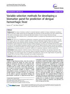
FIG. 3. Spectrum and selected intervals. (a) v ¼ 0.0; (b) v ¼ 0.7, d1 ¼ 5, d2 ¼ 30; (c) v ¼ 1.1, d1 ¼ 10, d2 ¼ 5; and (d) v ¼ 1.6, d1 ¼ 35, d2 ¼ 5.

training data. We may conclude that the threshold value of 1.1 can be used for predicting the weight fractions of two iron oxides (FeO and Fe2O3) when evaluating the MADs for training and test data. In this case, the number of measurement points reduces to about 30 percent of the total number of points and the measurement time required decreases accordingly. Still, the MAD for the test data is close to the case of using the whole spectrum and it is within an acceptable range when considering the standard error from the wet chemical analysis. Note that the unit of MAD is the same as the weight fraction of FeO or Fe2O3. If one is more concerned with the reduction of measurement points, some other cases having higher threshold values can be chosen. Table II and Fig. 3 show the selected intervals according to the specified sets of parameters. In Fig. 3 the solid lines at the bottom of the spectrum represent the intervals finally selected. Figure 4 shows scatter plots of the true weight fraction against the predicted weight fraction of FeO obtained from two different models with (v ¼ 0.0) and (v ¼ 1.1, d1 ¼ 10, d2 ¼ 5), respectively. Their corresponding R2 values are 0.9719 and 0.9419, respectively. As a result, we can conclude that the proposed procedure has superior performance in terms of

1402

Volume 61, Number 12, 2007

efficiency for variable selection as well as accuracy for predicting the weight fraction.

CONCLUSION In this paper, a novel statistical approach was proposed for the variable selection and the rapid determination of concentrations of chemical components using XRD measurement data. To build a calibration model, we employed a PLS regression model through leave-one-out cross-validation. It was shown that the number of measurement points can be reduced through the proposed variable selection procedure based on the VIP index, which saves measurement time with a small sacrifice of the predictive ability for a real on-line process. To evaluate the proposed procedure, it was applied to a real data set for determining weight fractions of FeO and Fe2O3 in iron ore. The performance of the proposed procedure was compared to the performance of existing methods such as PCR and stepwise regression models. The experimental results demonstrate that PLS is a more suitable regression technique than PCR and that the proposed procedure leads to a more accurate and efficient variable selection as compared to the stepwise regression method.

ACKNOWLEDGMENTS We would like to thank anonymous referees for their helpful comments. This work was supported by the Korean Science and Engineering Foundation through the National Core Research Center for Systems Bio-Dynamics at POSTECH.

FIG. 4. Scatter plots of the true weight fraction against the predicted weight fraction obtained from two models with (a) (v ¼ 0.0) and (b) (v ¼ 1.1, d1 ¼ 10, d2 ¼ 5). Squared correlation coefficients: R2(v¼0) ¼ 0.9719 and R2(v¼1.1) ¼ 0.9419.

1. G. Eng, L. May, A. Mills, A. Bober, and J. M. Adams, Appl. Spectrosc. 33, 384 (1979). 2. L. S. Zevin and G. Kimmel, Quantitative X-ray Diffractometery (SpringerVerlag, New York, 1995). 3. R. Jenkins and R. L. Snyder, Introduction to X-ray Powder Diffractometry (John Wiley and Sons, New York, 1996). 4. B. R. Bakshi and U. Utojo, Anal. Chim. Acta 384, 227 (1999). 5. P. Geladi and B. R. Kowalski, Anal. Chim. Acta 185, 1 (1986). 6. K.-S. Park, H. Lee, C.-H. Jun, K.-H. Park, J.-W. Jung, and S.-B. Kim, Chemom. Intell. Lab. Syst. 51, 163 (2000). 7. S. Wold, M. Sjo¨stro¨m, and L. Eriksson, Chemom. Intell. Lab. Syst. 58, 109 (2001). 8. L. Luo, X-Ray Spectrom. 35, 215 (2006). 9. Y. Wang, X. Zhao, and B. R. Kowalski, Appl. Spectrosc. 44, 998 (1900). 10. N. Nagata, P. G. Peralta-Zamora, R. J. Poppi, C. A. Perez, and M. I. M. S. Bueno, X-Ray Spectrom. 35, 79 (2006). 11. T. Artursson, A. Hagman, S. Bjo¨rk, J. Trygg, S. Wold, and S. P. Jacobsson, Appl. Spectrosc. 54, 1222 (2000). 12. T. V. Karstang and R. J. Eastgate, Chemom. Intell. Lab. Syst. 2 (1987). 13. I.-G. Chong and C.-H. Jun, Chemom. Intell. Lab. Syst. 78, 103 (2005). 14. L. Norgaard, A. Saudland, J. Wagner, J. P. Nielsen, L. Munck, and S. B. Engelsen, Appl. Spectrosc. 54, 413 (2000). 15. H. M. Heise, U. Damm, P. Lampen, A. N. Davies, and P. S. McIntyre, Appl. Spectrosc. 59, 1286 (2005). 16. KS Standard KS E 3013: Methods for determination of total iron content in iron ores (Korean Standards Association, 2001). 17. KS Standard KS E 3016: Methods for determination of ferrous oxide in iron ores (Korean Standards Association, 2003). 18. S. Wold, A. Ruhe, H. Wold, and W. J. Dunn III, SIAM J. Sci. Stat. Comput. 5, 735 (1984). 19. G. Derringer and R. Suich, J. Qual. Technol. 12, 214 (1980). 20. G. C. Derringer, Qual. Prog. 27, 51 (1994). 21. E. Vigneau, M. Devaux, E. Qannari, and P. Robert, J. Chemom. 11, 239 (1997). 22. N. Draper and H. Smith, Applied Regression Analysis (John Wiley and Sons, New York, 1981), 2nd ed. 23. G. H. Golub and C. F. van Loan, Matrix Computations (Johns Hopkins University Press, Baltimore, 1996), 3rd ed.

APPLIED SPECTROSCOPY

1403