A Variational Approach to the Modeling and ...

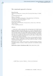
PROCEEDINGS, Thirty-Eighth Workshop on Geothermal Reservoir Engineering Stanford University, Stanford, California, February 11-13, 2013 SGP-TR-198

A VARIATIONAL APPROACH TO THE MODELING AND NUMERICAL SIMULATION OF HYDRAULIC FRACTURING UNDER IN-SITU STRESSES Chukwudi Chukwudozie1, Blaise Bourdin2 , and Keita Yoshioka3 1. Craft & Hawkins Department of Petroleum Engineering, Louisiana State University, Baton Rouge LA 70803, USA. Email: [email protected] 2. Department of Mathematics and Center for Computation & Technology, Louisiana State University, Baton Rouge LA 70803, USA. Email: [email protected] 3. Chevron Energy Technology Company, Houston TX 77002, USA. Email: [email protected]

ABSTRACT Most hydraulic fracturing simulation approaches apply propagation criteria to an individual fracture along prescribed path(s). In practice, however, the modeling of hydraulic fracturing in reservoir stimulation requires handling interactions between multiple natural or induced fractures growing along unknown paths, and changes in fracture pattern and network. In this paper, we extend the work of Bourdin et al 2012 and focus on the effectof in-situ stresses on crack path in 2D and 3D, and revisit the verification work against analytic solution with more realistic units. The approach is based on Francfort and Marigo's variational approach to fracture (Francfort and Marigo, 1998). The main idea is to recast Griffith's criterion for a single fracture growth into a global energy minimization problem. The energy we consider consists of the sum of surface and bulk terms accounting for the energy dissipated by a growing crack and the mechanical energy, including the work of residual (in-situ) stresses and pressure force against the fracture walls. To be more specific, we search the minimum of the total energy under any admissible fracture sets and kinematically admissible displacement field. Our focus is on quasi-static crack propagation propagation encountered during hydraulic fracturing process, which we model as a rate independent process. This approach does not need any a priori knowledge of the crack path, or any additional hypotheses concerning fracture nucleation or activation. We claim that it provides a mathematically rigorous and mechanistically sound unified framework accounting, derived from first principles, and accounting for new fractures nucleation, existing fractures activation, and full fracture path determination such as branching, kinking, and interaction between multiple cracks. It is no surprise that having no a priori hypothesis or knowledge on fracture geometry comes at the cost of numerical complexity. To overcome the complexities associating with handling of large and complex fracture patterns, we propose an

approach based on a regularized model where fractures are represented by a smooth function. In this paper, we first show series of comparison cases of the variational fracture simulation against analytical solutions. We demonstrate our approach's ability to predict complex behaviors such as turning fracture under in-situ earth stresses and the interactions of multiple fractures.

INTRODUCTION Hydraulic stimulation or high-pressure injection in geothermal reservoir often involves development of complex fractures due to the existence of natural fracture system and the relatively large thermal effects. However, conventional hydraulic fracture modeling assumes fracture propagation to be planar and perpendicular to the minimum principle stress (Adachi et al. 2007), which simplifies fracture propagation criteria to mode-I. Restricting propagation mode search into one direction and prescribing fracture growth plane can greatly reduce computation overhead but many of field observations, especially EGS experiment, suggest that fracture propagation is much more complex than planar (Fehler 1989; Asanuma et al. 2000; Gerard et al., 2006). To better describe complex responses from geothermal field, more tractable modeling approaches than ones derived from classical fracture mechanics have been increasingly applied such as smeared fracture or damage mechanics approach (Zhang et al., 2010) where computation elements turns to fractured mass when criteria are met, or reactivation of prescribed fractures and subsequent rock property modification (Moos and Barton, 2008; Rutqvist et al., 2008; McClure and Horne, 2011; Rutquivst). Similar efforts have been made in stimulation modeling in shale/tight gas (Mayerhofer et al. 2010) or waste injection (Moschovidis et al. 2000) to address predictive capabilities of complex fracture propagation (Rungamornrat et al. 2005; Gu et al. 2012; Hossain et al. 2000). This study is an extension of the previously proposed variational approach (Francfort and Marigo

1998, Bourdin et al. 2008) to hydraulic fracturing (Bourdin et al. 2012) accounting for the impact of insitu stresses on fracture propagation. One of the most appealing aspects of this approach is to account for arbitrary numbers of fractures in terms of energy minimization without any a priori assumption on their geometry, and without restricting their growth to specific grid directions. In this paper, we present early results obtained with this method. At this stage, our intent is not to implement all physical, chemical, thermal, and mechanical phenomena involved in the hydraulic stimulation process in geothermal reservoirs but to propose a mechanistically sound yet mathematically rigorous model and to demonstrate the its capabicity to predict propagation of fracture in an ideal albeit not unrealistic situation, for which we can perform rigorous analysis and quantitative comparison with analytical solutions. Specifically, we neglect all thermal and chemical effects and also assume that the fracturing stimulation is performed by hydraulic force not by explosives so that all inertial effects are negligible (quasi-static). Throughout the analyses presented, we consider reservoir as an impermeable perfectly brittle linear formation with no porosity and assume an inviscid fluid with no compressibility, which essentially lead to no leak-off to the formation and the constant fluid pressure inside the fracture (infinite fracture conductivity), depending only on the injected fluid volume and total fracture opening respectively. This setting is also known as toughness dominated case. THE VARIATIONAL APPROACH HYDRAULIC FRACTURING

TO

The foundation of most quasi-static brittle fracture models, is Griffith’s observation that the energy dissipation induced by a propagating crack has to be exactly offset by the decay of elastic energy. Typically, the latter is estimated in terms of the elastic energy restitution rate G, often derived from the stress intensity factors. In the Linear Fracture Mechanics framework, a branching criterion identifies crack path, based on the local stress configuration, or an energetic criterion, and propagation takes place when the elastic energy restitution rates reaches a critical value Gc. Noticing that the elastic energy restitution rate is often defined as the derivative of the total mechanical energy with respect to a crack increment length, Griffith’s criterion can be described in terms of the criticality of a total energy along a prescribed path. The basis of the variational approach to brittle fracture is to recast Griffith's criterion in a variational setting, i.e. as the minimization over any crack set (any set of curves in 2D or of surface in 3D, in the reference configuration) and any kinematically admissible displacement field u, of a total energy con-

sisting of the sum of the stored potential elastic energy and a surface energy proportional to the length of the cracks in 2D or their area in 3D. More specifically, consider a domain  in 2 or 3 space dimension, occupied by a perfectly brittle linear material with Hooke's law A and critical energy release rate (or fracture toughness) Gc. Let f(t,x) denote a time-dependent1 body force applied to , (t,x), a surface force applied to a part N of its boundary, and g(t,x) a prescribed boundary displacement on the remaining part D. To any arbitrary crack set  and any kinematically admissible displacement set u, we associate the total energy F ( u, G ) :=

ò W\G W ( e ( u)) dW - ò¶N W t × u ds -

ò W f × u dW + Gc H

N-1

( G)

,

(1)

where W is the elastic energy density associated with a linearized strain field e(u):=(u +Tu)/2, given by W(e(u)) := Ae(u), and HN-1() denotes the N-1 dimensional Hausdorff measure of  i.e. the length of  in two space dimensions and its surface area in three space dimensions. At any discrete time step ti, we look for the displacement field ui and the crack set I as the solution of the minimization problem: inf

u kinematically admissible     for all j  i j 

F u, 

Loosely speaking, minimality with respect to the displacement field accounts for the fact that the system achieves static equilibrium under its given crack set, optimality with respect to the crack set is a generalization of Griffith's stationarity principle G=Gc, and the growth constraint   j for any j < i accounts for the irreversible nature of the fracture process. At this point, we insist on the fact that the crack geometry itself is obtained through the energy minimization problem and not assumed known a priori or computed with an additional branching criterion, in contrast with most classical models. No assumption is made on the geometry of the crack set, other than the growth condition. In particular, one does not even assume that the crack set consists of a single curve or surface, or that the number of connected components remains constant during the evolution (which would preclude nucleation or merging). Indeed, one of the strengths of the variational approach is to provide a unified setting for the path determination, nucleation, 1

We follow a common abuse of language by referring to t as “time”. Rigorously, as we place ourselves in the context of quasi-static evolution, t is to be understood as an increasing loading parameter.

activation and growth of an arbitrary number of cracks in two and three space dimensions. The numerical implementation of Eq. 2 is a challenging problem that requires carefully tailored techniques. The admissible displacement fields are discontinuous, but the location of their discontinuities is not known in advance, a requirement of many classical discretization methods. Also, the surface energy term in Eq. 1 requires approximating the location of cracks, together with their length, a much more challenging issue. In particular, proper attention has to be paid to the issue of anisotropy induced by the grid (Chambolle, 1999) or the mesh (Negri, 1999) The approach we present here is based on the variational approximation by elliptic functional (Ambrosio and Tortorelli, 1990; Ambrosio and Tortorelli, 1992). A small regularization parameter  is introduced and the location of the crack is represented by a smooth “phase field” function v taking values 0 close to the crack and 1 far from them. More precisely, one can prove (see Braides, 1998; Chambolle, 2004; Chambolle, 2005) for instance) that as  approaches 0, the regularized energy Fe ( u, v ) := -

ò W v 2W ( e ( u)) dW - ò¶N W t × u ds

ò W f × u dW +

Gc 2

òW

(1 - v2 ) v2 + e Ñv 2 dW

(3)

e

traces of the displacement field. With these notations, the work of the pressure force p becomes then    pxu x  u x  xds ,

and

the

total

energy

becomes





Eu,  : F u,    px u  x  u  x   xds .(4)

Accounting for pressure forces in the regularized formulation is more technical, as the crack geometry is not tracked explicitly, but represented by the smooth field v. In the sequel, we propose to modify the regularized energy Eq. 3 and consider E u,  : F u,    pxux vxd .

(5)

Following the lines of the analysis carried out in (Chambolle, 2004b; Chambolle 2005), it can be proven that the -convergence property is preserved so that again, the minimizers of Eq. 5 converge to that of Eq.4. Intuitively, surface forces along the edges of  are replaced with properly scaled body forces applied in a neighborhood of the cracks. In the next sections, we illustrate some of the properties of this approximation and its ability to properly account for pressure forces and deal with unknown crack path, multiple cracks and changes in their topology.

approaches F in the sense of -converges, meaning that the minimizers of F converge as to that of F. NUMERICAL SIMULATIONS An important feature of the regularized problem, in view of its numerical implementation, is that it does not require an explicit representation of the crack network. Instead all computations are carried out on a fixed mesh and the arguments of F are smooth functions, which can be discretized with standard finite elements. Moreover, provided that the discretization size and regularization parameter satisfy some compatibility properties, it can be shown that the convergence property can be extended to the finite element discretization of F. The actual minimization follows the approach originally devised in (Bourdin, 1999; Bourdin et al., 2000; Bourdin, 2007) is achieved by alternating minimization with respect to the u and v fields, until convergence. The numerical implementation on parallel supercomputers uses the PETSc toolkit (Balay et al., 1997; Balay et al., 2012a; Balay et al., 2012b). Extension to hydraulic fracturing In order to adapt the variational fracture framework to hydraulic fracturing, one has to account for fluid pressure forces along the crack surfaces. For any point x on the crack set , we denote by  the oriented normal direction to  and by u+(x) and u-(x) the

We first revisit an idealized problem where a closed form solution can be obtained presented in (Bourdin et al, 2012). We consider an infinite two dimensional domain consisting of a homogeneous isotropic material with Young's modulus E and Poisson ratio  with a single pre-existing crack  of length 2l0 in the y=0 plane. Assuming that the displacement and stress fields vanish at infinity, it is then possible to derive an exact formula for the boundary displacement of the crack surface subject to a constant pressure force, under the plane-stress hypothesis (see Sneddon and Lowengrub, 1969, Sec 2.4, for instance). Setting E' = E/(1-2), we have that for  l0  x  l0 u  x,0 

12

2 pl0  x 2  1 E'  l0 2 

,

(6)

and that u  x,0  u  x,0 . From this, it is easy to derive that the total volume of the crack in the deformed configuration is

V=

2 p l02 . E'

(7)

The elastic energy restitution rate G can also be obtained by computing the work of the pressure forces for the displacement field in eq (6), deriving the total mechanical energy, and differentiating with respect to the crack length. Using this technique, one can easily see that if the pressure exceed the critical value Gc E' corresponding to an injected volp0  l0 4Gc l0 , then satisfying Griffith’s stabilE' ity criterion G=Gc becomes impossible. In the language of linear fracture mechanics, one says that the propagation becomes unstable. If one prescribes the injected volume V, however, it is easy to see that below the critical volume V0, the crack does not grow, and the pressure grows linearly until it reaches the critical pressure p0. When V exceeds V0, the crack grows and the pressure drops. The pressure and crack length are given by:

sistent with the compatibility condition for the convergence of the discretized regularized energy, which requires that h ≪ .

3

ume V0 

13

 2E' Gc  ,  V 

pV   

(10)

and 13

 E 'V 2  .   4Gc 

l V   

Figure 1: The v field associated with an injected volume of 2.5 the blue color corresponds to the value 1 (the uncracked material) and the red to 0 (the crack). The value of the regularization parameter ε is (left to right) 5.6E-2 (2.5h), 4.5E-2 (2h), 2.2E-2 (h), and 5.6E-3 (.25h). Qualitatively, one observes that the v field is a smooth function but becomes sharper as ε decreases.

(11)

As long as the crack remains short enough compared to the computational domain, one can expect that the solution obtained while forcing all components of the displacements to 0 at the boundary of the computational domain is close to that on an infinite domain described above. We ran a series of numerical simulations for a square domain of size 8 m  8 m with a horizontal crack of length .4 m in its center, discretized by a single layer of 355  355 bilinear finite elements of size h=2.25E-2 m and thickness 1E-2 m. Figure 1 represents the function v representing the crack set for an injected “volume” V=.025m2, and decreasing values of the regularization parameter . The color blue corresponds to the value 1, red to 0. As expected, one observes that the function v is smooth and remains close to 1 except on an area along a segment where it transitions to 0. Moreover, one sees that the width of the transition area decreases with . Figure 2 represents the the profile of the vfield along a cross section through x = 0 for the same value of h and various values of . We observe that if  is “too small” compared to the mesh size, the smooth profile is poorly approximated. This is con-

Figure 2:Profile of the v-field along the vertical cross-section x=4. Finally, Figure 3 compares the crack pressure and length as a function of the injected volume obtained for Young's modulus of 10 GPa and fracture toughness of 100 Pa-m with the closed form expressions Eqs. 10 and 11. When  is “too large”, the critical pressure is underestimated and the critical volume

overestimated. As the crack starts propagating, the computed length and pressures are very close to the exact expression. This behavior is explained by the softening taking place in the transition layer near the crack, which reduces the stresses near the crack tip. When  is “too small”, compared to the mesh size, the transition profile is poorly approximated, which leads to a poor approximation of the surface energy, hence of the crack length and pressure.

pressure, as expected. The approximation of the crack length also shows little sensitivity to the mesh size, and is very close to the expected value.

Figure 4: Effect of the discretization size on the injection pressure and crack length.

Figure 3: Pressure and crack length as a function of the injected volume. The solid lines correspond to different values of the regularization parameter , the dashed lines are the exact expressions given by (10) and (11). In Figure 5, we fixed the ratio  h and refined the mesh. Again, we observe that the approach is very robust in that the mesh size has almost no influence on the numerical solution. The pressure is slightly overestimated as the crack grows, which is expected given the choice of boundary condition. Indeed, we ran another series of experiments (not shown here) leaving the boundary of the computational domain stress free, which lead to slightly underestimating the

Isotropy of the discrete model The effect of mesh and grid isotropy on the approximation of free-discontinuity problems is now well understood (see Chambolle 1995, Negri 1999). The main issue is that the approximation of the surface energy associated with a unit length may exhibit a strong dependency on the crack orientation relative to the grid directions, when using structured meshes, and when the regularization parameter  is of the order of the mesh size. We reproduced the experiments from Figure 4 with a ratio  h of 2, starting from a crack forming an angle of 0, 15, 30, and 45 degrees with the x-axis. The evolution of the fluid pressure and crack length as a function of the injection volume are presented in Figure 6. The variations of the measured quantities due to the crack orientation are minimal, even for such a small e h ratio. Note that because of the finiteness of the computational domain,

some variations should be expected. A more careful study would be necessary in order to decouple the anisotropy due to the geometry of the computational domain from the one induced by its discretization. Note also that the results shown later in Figure 8 do not exhibit the classical artifact induced by an anisotropic approximation of the surface energy, i.e. cracks consisting solely of straight segments along the coordinate axes, but instead show cracks consisting of smooth curves.

o

and 15 (bottom row) with the horizontal axis, under uniaxial ( s 11 =50MPa, left) and biaxial in-situ stress fields ( s 11 =50MPa, s 33 =25MPa, right). Qualitatively, one observes that cracks reorient themselves along the vertical axis. As one would expect, the reorientation takes place within a smaller area when the domain is subject to uniaxial stresses. More surprisingly, for a shallow crack under uniaxial stress condition, asymmetric crack patterns are energetically favored over symmetric ones. Of course, the pattern displayed is one of two equivalent solutions. That our numerical algorithm favored one over the other is due to multiple factors including round-up error and numerical error of the iterative solvers for the alternate minimization algorithm, for instance. This example illustrates how even in the case of a symmetric problem, lack of uniqueness of the minimizer of the total energy can lead to a solution set consisting of multiple asymmetric solutions instead of a unique symmetric one. It also highlights how crack path identification can be complicated, even in the case of a very simple geometry. A better –quantitative– comparison with classical solutions is pending and was not available in time for inclusion in this report. Again, we stress that the fact that the pre-existing cracks propagate in the direction orthogonal to the least principal stress arises from the energy minimization principle, and is not enforced explicitly.

Figure 5: Evolution of the injection pressure and crack length for cracks with angles of 0,15,30,45 degrees from the x-axis. Effect of in-situ stresses It is well known that during hydraulic fracturing, an isolated crack will reorient itself until it becomes orthogonal to the direction of least principal stress (Weng 1993, Adachi et al. 2007). We repeated the previous series of computation while subjecting the computational domain to boundary forces simulating in-situ stresses. Figure 6 represents the evolution of a o pre-existing crack forming an angle of 30 (top row)

Figure 6: Crack path for a slanted crack under insitu stresses. Fracture propagation under prescribed injection rate in 3D The same analysis can be carried out in three space dimension in which case, the critical pressure p0 and injected volume V0 associated with a pre-existing penny shape crack of radius R0 are

Gc E'  , 4R0

(12)

64Gc R0 . 9E'

(13)

p0 

and 5

V0 

Just as in the two dimensional case, it is possible to show that as long at V < V0, the crack does not grow, and that for V > V0, the crack radius and pressure are given by 15

 Gc 3 E' 2  3   ,  12V 

pV   

(14)

and 15

 9 E 'V 2  .   64Gc 

RV   

We ran a series of three dimensional experiments on a cubic domain 10 m  10 m  10 m discretized using various resolution ranging from 50  50  50 to 250  250  250 bilinear finite elements. The Young's modulus is 10 GPa, and the fracture toughness is 191 Pa-m. We account for a pre-existing penny shape crack of radius R0 = 1 m in the plane x = 5 by building the v-field given by Eq. 8, and prescribe to 0 all components of the displacement field on the boundary of the domain. Figure 7 shows the evolution of the fluid pressure and crack surface area as a function of the injected volume, compared with different resolutions. The discrepancy in the surface energy for small injected volume of fluid is due to the way the initial crack is constructed as an approximation of the v field associated with a penny-shaped crack, but seems to bear no impact on the crack evolution for higher injection volume.

(15) Again, the impact of in-situ stresses on crack path can be studied by repeating the same computation with while varying the orientation of the initial crack. We started from a crack with normal vector forming an angle φ with the vertical axis (co-latitude) and θ with the x-axis (longitude), and varied the form of the in-situ stress field

Figure 8: Crack path for a single slanted pennyshaped crack propagating under prescribed injection volume in a medium subject to anisotropic in-situ stresses.

Figure 7: Pressure and crack radius as a function of the injected volume. Numerical simulations (solid lines) and closed form solution (14-15) (dashed line).

Figure 8 show the crack pattern (obtained by taking the isosurface 0.1 of the v field). The first row correspond to an initial crack orientation φ=30˚, θ=10˚ and a stress field given by σ11=-50MPa, σ22=-25MPa, and σ33=-50MPa (left) and σ11=-5MPa, σ22=50MPa, and σ33=-50MPa (right). The second row corresponds to orientation φ=30˚, θ=0˚, and σ11=5MPa, σ22=-50MPa, and σ33=-50MPa (left) or σ11=-50MPa, σ22=-5MPa, and σ33=-50MPa (left). . As in the two-dimensional case, we observed that asymmetric propagation is sometimes favored of symmetric one, and that the area within which crack change direction is affected by the anisotropy of the in-situ stress field. A quantitative study of this phenomenon is pending. Interaction between two pressurized cracks in 2D Beside its ability to identify complex crack paths in 2 and 3 dimension, the variational approach to fracture is also capable of handling interactions between cracks in a simple and efficient way, which we illustrate in a final set of numerical experiments. In a twodimensional setting, we consider the problem of two pressurized cracks close enough from each other to interact: in a square domain  = 8m  8m, we placed two straight cracks of length 1m, centered at (3.,4.25) and (4.8,4.75) and with polar angle 0 and ‑30o. For the sake of simplicity, we only prescribed the total injected volume, and assumed that the pressure was constant and equal in each crack.

length as a function of the injected volume. The system evolves as follows: 1. For V < 3.3E-2 m2, neither of the cracks propagate. As in the case of a single crack, the pressure grows as a linear function of the injected volume. 2. Upon a first critical volume V  3.3E-2 m2, one of the crack tip activates. A crack grows along a curved path, heading towards the second crack. As expected, as a crack propagates, the fluid pressure drops. The critical pressure is p  .066 MPa, compared to p0  .79 MPa for an isolated crack with the same length. 3. When V  5.6E-2 m2, the cracks connect. Notice that the handling of the crack merging requires no additional work in the variational approach. 4. From V  5.6E-2 m2 until V  6.8E-2 m2, the pressure grows linearly, and the crack length remains constant; 5. Finally, after V  6.8E-2 m2, another crack tip activates, and we observe again a pressure drop. We insist again that in this and the above simulations, the crack path was not precomputed or enforced through a branching criterion. Instead it was obtained by minimization of the system’s total energy. Even changes in crack topology were handled transparently by the regularized model and required no additional processing. Finally, in the variational approach, handling multiple interacting cracks or interactions with pre-existing cracks is no more complicated or computationally intensive that handling a simple crack.

CONCLUSIONS Through a series of simple numerical verification experiments, we show how the variational approach to fracture can address some of the challenges encountered in the numerical simulation of hydraulic stimulation, including the identification of complex crack path in 2 and 3 dimensions, the handling of insitu stresses, and the interactions between multiple cracks. So far, most of our effort has been focused on verification numerical experiments under very idealized situations. A next phase of this work will focus on the validation of the model and its implementation against real experiments. Further extensions will also be required in order to handle flow in the reservoir and leak-off, for instance.

Figure 9: Evolution of crack geometry. Snapshot of the v field for an injected volume of .033, .056, .068, and .01 m2. The evolution of the crack path, using the same convention as before is shown in Figure 9, while Figure 10 highlight the evolution of the pressure and crack

ACKNOWLEDGEMENTS The authors wish to thank P. Connolly and T. Buchmann of Chevron for stimulating discussions concerning the variational approach to fracture and Chevron management for permission to publish this work. This material is based in part upon work supported by Chevron under "Variational fracture approach to reservoir stimulation" (C. Chukwudozie

and B. Bourdin) and the National Science Foundation under Grants No. DMS-0909267 (B. Bourdin). Some of the numerical simulations were performed using resources from the Extreme Science and Engineering Discovery Environment (XSEDE), supported by National Science Foundation grant number OCI1053575, and provided by TACC at the University of Texas.

Figure 10: Evolution of the pressure (left) and total crack length (right) for two interacting cracks.

REFERENCES Adachi, J., E. Siebrits, A. Peirce, and J. Desroches. 2007. “Computer Simulation of Hydraulic Fractures.” Int. J. Rock Mech. & Min. Sci. 44 (02): 739–757. Ambrosio, L., and V.M. Tortorelli. 1990. “Approximation of functionals depending on jumps by elliptic functionals via Γ-convergence.” Comm. Pure Appl. Math. 43 (8): 999–1036.

Ambrosio, L., and V.M. Tortorelli.. 1992. “On the approximation of free discontinuity problems.” Boll. Un. Mat. Ital. B (7) 6 (1): 105–123.‑ Asanuma, H. et al. 2004. “Microseismic Monitoring of a Stimulation of HDR Reservoir at Cooper Basin, Australia, by the Japanese Team” Geothermal Resources Council 28: 191-195.‑ Balay, S., J. Brown, , K. Buschelman, V. Eijkhout, W.D. Gropp, D. Kaushik, M.G. Knepley, L.C. McInnes, B.F. Smith, and H .Zhang. 2012a. “PETSc Users Manual.” Technical Report ANL95/11 - Revision 3.3, Argonne National Laboratory. Balay, S., J. Brown, K. Buschelman, W.D. Gropp, D.Kaushik, M.G. Knepley, L.C. McInnes, B.F. Smith, and H. Zhang. 2012b. PETSc Web page. http://www.mcs.anl.gov/petsc. Balay, S., W.D. Gropp, L.C. McInnes, and B.F. Smith. 1997. “Efficient Management of Parallelism in Object Oriented Numerical Software Libraries.” Edited by E. Arge, A. M. Bruaset, and H. P. Langtangen, Modern Software Tools in Scientific Computing. Birkh ‑auser Press, 163– 202. Bourdin, B. 1999. “Image segmentation with a finite element method.” M2AN Math. Model. Numer. Anal. 33 (2): 229–244. Bourdin, B. 2007. “Numerical implementation of a variational formulation of quasi-static brittle fracture.” Interfaces Free Bound. 9 (08): 411– 430.‑ Bourdin, B., G.A. Francfort, and J.-J. Marigo. 2000. “Numerical experiments in revisited brittle fracture.” J. Mech. Phys. Solids 48 (4): 797–826.‑ Bourdin, B., G.A. Francfort, and J.-J. Marigo. 2008. “The Variational Approach to Fracture.” J. Elasticity 91 (1-3): 1–148. Bourdin, B., C. Chukwudi, and K. Yoshioka. 2012. “A Variational Approach to the Numerical Simulation of Hydraulic Fracturing” Proceedings of the 2012 SPE Annual Technical Conference and Exhibition. SPE 146951. Braides, A. 1998. Approximation of FreeDiscontinuity Problems. Lecture Notes in Mathematics no. 1694. Springer. Burke, S., C. Ortner, and E. Süli. 2010. “An adaptive finite element approximation of a variational model of brittle fracture.” SIAM J. Numer. Anal. 48 (3): 980–1012.‑ Chambolle, A. 1999. “Finite-differences discretizations of the Mumford-Shah functional.” M2AN Math. Model. Numer. Anal. 33 (2): 261–288. Chambolle, A. 2004. “An approximation result for special functions with bounded variations.” J. Math Pures Appl. 83:929–954. Chambolle, A. 2005. “Addendum to “An Approximation Result for Special Functions with Bounded Deformation” [J. Math. Pures Appl. (9) 83 (7) (2004) 929–954]: the N-dimensional case.” J. Math Pures Appl. 84:137–145.

Fehler, M. 1989. “Stress Control of Seismicity Patterns Observed during Hydraulic Fracturing Experiments at the Fenton Hill Hot Dry Rock Goethermal Energy Site, New Mexico.” Int. J. Rock Mech. and Min. Sci. 26 (3): 211-219. Francfort, G.A., and J.-J. Marigo. 1998. “Revisiting brittle fracture as an energy minimization problem.” J. Mech. Phys. Solids. 46 (8): 1319–1342. Gerard, A. et al. 2006. “The deep EGS (Enhanced Geothermal System) project at Soultz-sousForets (Alsace, France).” Geothermics 35: 473483. Gu, H., J. Weng, J. Lund, U. Mack, M. Ganguly, and R. Suarez-Rivera. 2012. “Hydraulic Fracture Crossing Natural Fracture at Nonorthogonal Angles: A Criterion and its Validation.” SPEPO SPE 139984 (Feb): 20–26. Hossain, M.M., M.K. Rahman, and S.S. Rahman. 2000. “Volumetric Growth and Hydraulic Conductivity of Naturally Fractured Reservoirs During Hydraulic Fracturing: A Case Study using Australian Condictions.” Proceedings of the 2000 SPE Annual Technical Conference and Exhibition. SPE 63173. Mayerhofer, M.J., E.P. Lolon, N.R. Warpinski, C.L. Cipolla, D. Walser, and C.M. Rightmire. 2010. “What Is Stimulated Reservoir Volume?” SPEJ SPE 119890 (02): 89–98. Mayerhofer, M.J., E.P. Lolon, J.E. Youngblood, and J.R. Heinze. 2006. “Integration of Microseismic Fracture Mapping Results with Numerical Fracture Network Production Modeling in the Barnett Shale.” Proceedings of the 2006 SPE Annual Technical Conference and Exhibition. SPE 102103. McClure, M.W. and Horne, R.N. 2012. “Investigation of Injection-Induced Seismicity using a Coupled Fluid Flow and Rate and State Friction Model.” Geophysics. 76 (6): 181-198. Moschovidis, Z., R. Steiger, R. Peterson, N. Warpinski, C. Wright, E. Chesney, J. Hagan, A. Abou-Sayed, R. Keck, M. Frankl, C. Fleming, S. Wolhart, B. McDaniel, A. Sinor, S. Ottesen, and Miller. 2000. “The Mounds Drill-Cuttings Injection Field Experiment: Final Results and Conculusions.” Proceeding of the 2000 IADC/SPE Drilling Conference, SPE 59115. Moos, D. and Barton, C.A. 2008. “Modeling uncertainty in the permeability of stress-sensitive fractures.” The 42nd US Rock Mechanics Symposium, June 29 – July 2, San Francisco, CA Negri, M. 1999. “The anisotropy introduced by the mesh in the finite element approximation of the Mumford-Shah functional.” Numer. Funct. Anal. Optim. 20 (9-10): 957–982. Rungamornrat, J., M.F. Wheeler, and M.E. Mear. 2005. “A Numerical Technique for Simulating Nonplanar Evolution of Hydraulic Fractures.” Proceedings of the 2005 SPE Annual Technical Conference and Exhibition. SPE 96968.

Rutqvist, J., Birkholzer, J.T., and Tsang, C.-F. 2008. “Coupled reservoir-geomechanical analysis of the potential for tensile and shear failure associated with CO2 injection in multilayered reservoir-caprock systems.” Int. J. Rock Mech. and Min. Sci. 45: 132-143. Sneddon, I.N., and M. Lowengrub. 1969. Crack problems in the classical theory of elasticity. The SIAM series in Applied Mathematics. John Wiley & Sons. Weng, X. “Fracture Initiation and Propagation From Deviated Wellbores.” 1993. Proceedings of the 1993 SPE Annual Technical Conference and Exhibition. SPE 26597. Zhang, Z.Z. “Three-dimensional fracture simulation using the virtual multidimensional internal bond.” 2010. 44th US Rock Mechanics