A VECTORIAL VARIATIONAL MODE SOLVER AND ITS APPLICATION TO PIECEWISE CONSTANT AND DIFFUSED WAVEGUIDES O. (Alyona) Ivanova, Remco Stoffer, Manfred Hammer, E. (Brenny) van Groesen University of Twente, MESA+ Institute for Nanotechnology, P.O. Box 217, 7500 AE Enschede, The Netherlands
[email protected] Abstract – A Variational Vectorial Mode Solver for 3-D dielectric waveguides with arbitrary 2-D crosssections is proposed. It is based on expansion of each component of a mode profile as a superposition of some a priori defined functions defined on one coordinate axis times some unknown continuous coefficient functions, defined on the other axis. By applying a variational restriction procedure the unknown coefficient functions are determined as an optimum approximation of the true vectorial mode profile. A couple of examples illustrate the performance of the method. I.
I NTRODUCTION
Optical waveguides are main ingredients in many integrated optical circuits, and design tools for these waveguides are of great importance. Detailed overviews of such techniques are presented in [1, 2]. In this paper we extend the scalar Variational Mode Expansion Method [3] to fully vectorial simulations of lossless isotropic dielectric waveguides with – in principle – arbitrary refractive index distribution. The validity of the method is checked for a waveguide with non-rectangular piecewise-constant refractive index distribution and a diffused waveguide. II.
VARIATIONAL V ECTORIAL M ODE S OLVER
A. Problem Formulation Consider a z-invariant dielectric isotropic waveguide defined on its cross-section by a refractive index distribution n(x, y). Given the frequency ω we are looking for a solution of the Maxwell equations in the form of a field which propagates harmonically along the z-axis with propagation constant β: ¯ E(x, y, z) = E(x, y)e−iβz ,
¯ H(x, y, z) = H(x, y)e−iβz .
Solutions of this form correspond to stationary points of the functional [4] β= with
ωε0 hE, εEi + ωµ0 hH, Hi + ihE, CHi − ihH, CEi , hE, RHi − hH, REi
0 1 0 R = −1 0 0 , 0 0 0
0 C= 0 −∂y
0 0 ∂x
∂y −∂x , 0
(1)
(2)
R vacuum permittivity ε0 , vacuum permeability µ0 , ε = n2 (x, y), and the inner product hA, Bi = A∗ · B dx dy. The natural interface conditions are the continuity of all tangential field components across discontinuity lines. B. Modal Field Ansatz In this method each field component F ∈ {Ex , Ey , Ez , Hx , Hy , Hz } is represented individually as a superposition of nF a priori known functions XjF (x), defined on one coordinate axis, times some unknown coefficient-function YjF (y), defined on the other axis: F (x, y) =
nF X
XjF (x)YjF (y).
(3)
j=1
It is usually a matter of experience and intuition to guess a most adequate trial field XjF (x). Similar to the Film Mode Matching method [5] or to the Effective Index approach [6], in this paper XjF (x) was taken to be an appropriate component of a (1-D) mode of a particular constituting slab waveguide. Note, however, that the corresponding function YjF (y) contributes on the entire lateral axis.
C. Solution By restricting the functional (1) to the field template (3) one obtains a system of first order differential equations for the unknown continuous functions YF (a vector function consisting of all the functions YjF (y)), with β as a parameter. It turns out that it is possible to eliminate the functions YEy , YEz , YHy and YHzµto reduce the ¶ YEx (y) problem to a system of second order differential equations for only the unknown function u(y) = YHx (y) and parameter β of the form S1 u + (S2 u0 + βS3 u)0 = β 2 S4 u + βS5 u0
(4)
with continuity conditions across the interfaces for u and S2 u0 + βS3 u. The elements of the matrices Si consist of overlap integrals between functions XjF (x), their derivatives, and the permittivity distribution. So in general they also depend on y. In case the refractive index distribution n(x, y) is piecewise constant along the y-axis, one can define slices, such that inside each of these slices the matrices Si are constant along y. Provided that the field components Ey and Ez , and also Hy and Hz are approximated by the same functions, then in the each slice S2 = S4 and S3 = S5 and (4) becomes S1 u + S2 u00 = β 2 S2 u. (5) Moreover the matrices S1 and S2 are block-diagonal in such a way that equations for functions YEx and YHx decouple inside the slices; coupling occurs only across the vertical interfaces. By solving the system of second order differential equations with constant coefficients (5) inside each slice and by matching the solutions across interfaces, one arrives at a nonlinear eigenvalue problem in β. Iterations are required to find all β’s. In case of an arbitrary refractive index distribution the matrices Si do depend on y. In this case we choose a Finite Element Method to solve (4). One obtains a quadratic eigenvalue problem in β. All β values are found automatically from the numerical solution of the eigenvalue problem. This can be very useful if one wants to expand a field in terms of waveguide modes, as e.g. in [7, 8]. III.
N UMERICAL R ESULTS
To show the flexibility of this method we apply it first to a diffused waveguide [9] with a refractive index distribution given by ½ 2 ns + n2s (1.052 − 1) exp(−x2 /16) exp(−y 2 /4), if x > 0; n2 (x, y) = (6) n2c , if x < 0, where n2s = 2.1, n2c = 1.0 and λ = 1.3 µm. The results are summarized in Fig. 1. 1.5 7 6
1.4
x (µm)
5 1.3
4
n
3
1.2
2 1
1.1
0 1
a)
−6
−4
−2
0 y (µm)
2
4
6
b)
Fig. 1: a) Refractive index distribution n(x, y) of the diffused waveguide (6). b) Field profiles of the dominant electric component Ey of the fundamental TE mode. A computational window (x, y) ∈ [−1, 8]×[−6, 6] µm2 together with an approximation (3) of each field component by 1 (left picture) and 15 (right picture) functions and 20 elements in the finite element scheme were used. The effective index Neff = 2πβ/λ of the fundamental mode on the left picture is 1.4965 and on the right 1.48802, which compares well with a rigorous Finite Difference simulation (with 129 × 129 grid points) [11] 1.48797. Note that with a rough approximation by one function a reasonable estimation of the propagation constant and field profile is achieved, although for more rigorous analysis more functions are needed.
Next we consider a waveguide with piecewise constant non-rectangular refractive index distribution [10].
Fig. 2: Vectorial field profile of the fundamental mode of the slanted sidewall InP / InGaAsP polarization rotator from [10]. The top and bottom layers are InP, index 3.17; the middle layer and the outgoing slab are InGaAsP, index 3.27; cover: air, index 1.0. The maximum thickness of the InGaAsP layer is 1.3 µm; its minimum thickness is 0.1 µm. The top InP cap layer is 0.5 µm thick. The angle between the horizontal and the slanted sidewall is 52 degrees. The width at the top of the structure is 1.15 µm; the vacuum wavelength is 1.55 µm. A computational window (x, y) ∈ [−2, 2.5] × [−2, 3.5] µm2 with an approximation (3) of each field component by 7 functions and 50 elements in the finite element scheme were used. Already with such a low number of functions the effective index of the fundamental mode Neff = 2πβ/λ = 3.2223 agrees remarkably well with that of a rigorous Film Mode Matching simulation (with 320 modes and 50 slices) of [11] Neff = 3.2225.
IV.
C ONCLUDING R EMARKS
A variational method for the fully vectorial analysis of arbitrary isotropic dielectric waveguides was developed. Similar to the scalar approach [3] this method gives rather accurate estimates of the propagation constants, sometimes even with only a few terms in the expansion. Similar ideas can in principle be applied to scattering problems in 3D. ACKNOWLEDGMENT This work was supported by the Dutch Technology foundation (BSIK / NanoNed project TOE.7143). R EFERENCES [1] K.S. Chiang. Review of numerical and approximate methods for the modal analysis of general optical dielectric waveguides. Optical and Quantum Electronics, 16, S113-S134 (1994). [2] R. Scarmozzino, A. Gopinath, R. Pregla and S. Helfert. Numerical techniques for modelling guided wave photonic devices. J. Sel. Topics Quantum Electron. 6(1), 150-162 (2000). [3] O.V. Ivanova, M. Hammer, R. Stoffer and E. van Groesen. A variational mode expansion mode solver. Optical and Quantum Electronics, 39, 849–864 (2007). [4] C. Vassallo. Optical Waveguide Concepts. Elsevier, Amsterdam, 1991. [5] A.S. Sudbø. Film mode matching: a versatile numerical method for vector mode field calculation in dielectric waveguides. Pure Appl. Opt. 2, 211-233 (1993). [6] R. M¨arz, Integrated optics design and modelling, Artech house, Boston, London (1994). [7] M. Hammer. Hybrid analytical/numerical coupled-mode modeling of guided wave devices. Journal of Lightwave Technology, 25 (9), 2287–2298 (2007). [8] R. Stoffer, A. Sopaheluwakan, M. Hammer and E. van Groesen. Helmholtz solver with transparent influx boundary conditions and nonuniform exterior. In proc. of XVI International Workshop on Optical Waveguide Theory and Numerical Modelling, Copenhagen, Denmark; book of abstracts 3 (2007). [9] A. Sharma, P. Bindal. An accurate variational analysis of single-mode diffused waveguides. Optical and Quantum Electronics, 24, 1359– 1371 (1992). [10] S.S.A. Obayya, N. Somasiri, B.M.A. Rahman and K.T.V. Grattan. Full vectorial finite element modeling of novel polarization rotators. Optical and Quantum Electronics, 35, 297–312 (2003). [11] FieldDesigner by http://www.phoenixbv.com/.