A variational mode solver for optical waveguides based on quasi

A variational mode solver for optical waveguides based on quasi-analytical vectorial slab mode expansion Alyona Ivanova1 , Remco Stoffer1,2 , and Manfred Hammer1 1

MESA+ Institute for Nanotechnology, University of Twente, Enschede, The Netherlands 2 PhoeniX Software, Enschede, The Netherlands

A flexible and efficient method for fully vectorial modal analysis of 3D dielectric optical waveguides with arbitrary 2D cross-sections is proposed. The technique is based on expansion of each modal component in some a priori defined functions defined on one coordinate axis times some unknown coefficient-functions, defined on the other axis. By applying a variational restriction procedure the unknown coefficient-functions are determined, resulting in an optimum approximation of the true vectorial mode profile. This technique can be related to both Effective Index and Mode Matching methods. A couple of examples illustrate the performance of the method. Keywords: Integrated optics; Dielectric waveguides; Guided modes; Numerical modelling; Variational Methods PACS : 42.82.m; 42.82.Et

1

Introduction

Three-dimensional optical channel waveguides are basic components of integrated optical devices such as directional couplers, wavelength filters, phase shifters, and optical switches. The successful design of these devices requires an accurate estimation of the modal field profiles and propagation constants. Over already some decades several classes of methods for the analysis of dielectric optical waveguides were developed: among these are techniques of more numerical character, like Finite Element and Finite Difference approximations, the Method of Lines, and Integral Equations Methods, but also more analytical approaches like Film Mode Matching (FMM) and the Effective Index Method (EIM). Detailed overviews of these techniques can be found in [1, 2, 3]. In the present paper we propose an extension of the scalar mode solver [4] to vectorial problems. Our method is based on individual expansions of each mode profile component into a set of a priori defined functions of one coordinate axis (vertical), here, field components of some slab waveguide mode. The expansion is global, meaning that the same basis functions are used at any point on the horizontal axis. The unknown expansion coefficients – in our case functions, defined on the horizontal axis – are found by means of variational methods [5, 6]. The present method can be viewed as some bridge between two popular approaches, namely the FMM on the one hand and the EIM on the other. In the standard EIM the 2D problem of finding modes of the waveguide is reduced to consecutive solving two 1D problems: at first, the 1D modes, and their propagation constants, of the constituting slab waveguides are found, and then their propagation constants are used to define effective refractive indices of a reduced 1D problem. In general this is a very quick and easy approach for a rough estimation of mode parameters. However, in case one of the constituting slabs doesn’t support a guided mode (for example, some substrate material with air on top) it is impossible to uniquely define the effective refractive index in that particular region of the reduced problem. Should it be the refractive index of the cladding,

1

refractive index of the air, or something in between? The restriction of the present approach to one-term expansions will answer this question. The validity of the method was checked on several structures, including waveguides with rectangular and non-rectangular piecewise-constant refractive index distributions, and a diffused waveguide. Comparison shows that the present method is a more consistent and accurate alternative to the standard EIM and also can be pushed to its limits and used for rigorous computations. The paper is organized as follows. In section 2 the problem of finding vectorial modes of the dielectric waveguides is stated, then some properties of slab modes and the modal field ansatz are described in sections 3 and 4. The equations for the coefficient functions are derived in section 5. Section 6 outlines the numerical solution methods. The relation of the present method to the EIM and FMM is explained in more detail in sections 7 and 8. Then in section 9 numerical results for several waveguide configurations are presented. Finally some concluding remarks are made in section 10.

2

Variational form of the vectorial mode problem

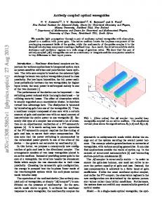
Consider a z-invariant dielectric isotropic waveguide defined on its cross-section by a refractive index n(x, y) or relative dielectric permittivity ε(x, y) = n2 (x, y) distribution. Figure 1 shows two examples. Figure 1: Examples for 3D dielectric waveguides defined on their cross-section by permittivity distribution ε(x, y). The structures are invariant along the z-axis. (a) box-shaped hollow-core waveguide, a concept from [7], the subject of section 9.1, (b) a standard rib waveguide, investigated in section 9.2.

¯ and magnetic H ¯ components of The propagation of monochromatic light, given by the electric E the optical field, with propagation constant β and frequency ω, ¯ E(x, y, z, t) = E(x, y) e−i βz ei ωt ,

¯ H(x, y, z, t) = H(x, y) e−i βz ei ωt ,

(1)

is governed by the Maxwell equations for the mode profile components E and H ωε0 εE + i CH = βRH, ωµ0 µH − i CE = −βRE, with



 0 1 0 R =  −1 0 0  , 0 0 0



 0 0 ∂y 0 −∂x  , C= 0 −∂y ∂x 0

(2)

(3)

vacuum permittivity ε0 , vacuum permeability µ0 , relative permittivity ε(x, y) = n2 (x, y). Here and further in this paper it is assumed that the relative permeability µ is equal to 1, as is the case for most materials at optical frequencies. We will work with a variational formulation of the Maxwell equations. Solutions (β, E, H) of the equations (2) correspond to stationary points (E, H) of the functional [5] F(E, H) =

ωε0 hE, εEi + ωµ0 hH, Hi + i hE, CHi − i hH, CEi , hE, RHi − hH, REi

(4)

with propagation constant β = F(E, H) equal R ∗ to the value of the functional at the stationary point. The inner product used is hA, Bi = A · B dx dy. The natural interface conditions are the continuity of all tangential field components across the interfaces.

2

3

Slab modes

In this section we will consider modes of slab waveguides, which we will use in the next section as building blocks to construct approximations of the modes of waveguides with arbitrary 2D crosssections. Furthermore, we introduce rotations of the slab modes; these rotations will be needed to provide a physical motivation for the particular form of the approximations that we will employ.

Figure 2: A slab waveguide with permittivity distribution εr (x) and principal component χEy of a corresponding TE slab mode (5).

A one dimensional TE mode, propagating in the z-direction with propagation constant βr,TE , of the slab waveguide, given by the permittivity distribution εr (x) (Figure 2) can be represented as     0 0, χEy (x), Ex , Ey , Ez (x, y, z) = e−i βr,TE z . (5) Hx , Hy , Hz 0, χHz (x) χHx (x), The principal electric component χEy satisfies the equation
′′ χEy (x) + k2 εr (x)χEy (x) = βr,2 TE χEy (x)

(6)

with vacuum wavenumber k = 2π/λ. The remaining two nonzero components of the mode profile can be derived directly from χEy :
′ βr,TE Ey i (7) χHz (x) = χ (x), χEy (x) . ωµ0 ωµ0 The slab waveguide (Figure 2) is by definition invariant in the (y, z)-plane. So if a modal solution of Maxwell equations propagating in the z-direction will be rotated in the (y, z)-plane by an angle θ (Figure 3), it will still remain a modal solution of the Maxwell equations, but now propagating in the direction (y, z) = (− sin θ; cos θ):     Ex , Ey , Ez 0, χEy (x) cos θ, χEy (x) sin θ (x, y, z) = e−i βr,TE (− sin θy + cos θz) . Hx , Hy , Hz χHx (x), −χHz (x) sin θ, χHz (x) cos θ (8) χHx (x) = −

Figure 3: A slab TE (TM) mode propagating in the z-direction with propagation constant βr,TE (TM) is rotated around the x-axis by an angle θ. The rotated mode propagates with the same propagation constant, but in the direction (y, z) = (− sin θ, cos θ). Similarly a 1D TM slab mode, propagating in the z-direction with propagation constant βr,TM    E  0, χEz (x) Ex , Ey , Ez χ x (x), (x, y, z) = e−i βr,TM z , (9) Hx , Hy , Hz 0 0, χHy (x), will still be a solution of the Maxwell equations after a rotation around the x-axis (Figure 3)    E  χ x (x), −χEz (x) sin θ, χEz (x) cos θ Ex , Ey , Ez e−i βr,TM (− sin θy + cos θz) . (x, y, z) = 0, χHy (x) cos θ, χHy (x) sin θ Hx , Hy , Hz (10) 3

The principal magnetic component χHy satisfies the equation  ′ 1 1 ′ Hy (χ (x)) + k2 χHy (x) = βr,2 TM χHy (x). εr (x) εr (x)

(11)

Again the remaining two nonzero components of the mode profile can be derived directly from χHy : χEx (x) =

4

βr,TM χHy (x), ωε0 εr (x)

χEz (x) = −


′ i χHy (x) . ωε0 εr (x)

(12)

Modal field ansatz

We now return to the vectorial modes of the 3D waveguides, as in section 2. Each field component F ∈ {Ex , Ey , Ez , Hx , Hy , Hz } is represented individually as a superposition of mF a priori known functions XjF (x), defined on one coordinate axis, times some unknown coefficient-function YjF (y), defined on the other axis: mF X F (x, y) = XjF (x)YjF (y). (13) j=1

For the functions X we will take components of slab modes from some reference slice(s). Further in the paper two types of the expansion will be relevant, one which introduces 5 unknown functions Y per slab mode, and another one, which introduces only 3. These will be called five component approximation (VEIM5) and three component approximation (VEIM3), respectively. E x In case of VEIM5, the TE basis mode (5) number j with mode profile components χj y , χH j , E

E

z χH contributes to the expansion of components Ey , Ez , Hx , Hy and Hz with the form χj y Yj y , j

E

Hy

Hx Hz x χj y YjEz , χH j Y j , χj Y j

Hz z and χH j Yj . Likewise, the TM basis mode (9) number l with mode

E

Hz x contributes to the expansion of components Ex , Ey , Ez , Hy and profile components χl y , χH l , χl Hy Hz Hy Hy Ez Ez Ey Ex Ex z Hz with the form χl Yl , χl Yl , χE l Yl , χl Yl , χl Yl , such that the complete expansion looks like !   E E E P 0, χj y (x)Yj y (y), χj y (x)YjEz (y) Ex , Ey , Ez (x, y, z) = + Hy Hx Hz Hz Hz x Hx , Hy , Hz χH j∈TE j (x)Yj (y), χj (x)Yj (y), χj (x)Yj (y) (14) ! Ey Ez Ez Ez Ex x P (y) (x)Y (y), χ (x)Y (y), χ (x)Y χE l l l l l l . + H H H 0, χl y (x)Yl y (y), χl y (x)YlHz (y) l∈TM

This expansion has the drawback that the functions making up some of the components can H become linearly dependent; for example, the full set of χl y (x) components from TM modes form a z complete set; thus any χH j (x) from a TE mode can be expressed in that complete set of functions. When using a limited number of modes in the expansion, no problems result from this; however, increasing the number of modes will at some point make the problem ill-conditioned. Therefore, we introduce a different expansion, which we call VEIM3, in which we omit contributions of some modal components - making sure that each vector component is only represented by either TE of TM slab mode components. So a TE basis mode (5) number j with mode profile components E Ey Ey Hz x χj y , χH j , χj contributes to the expansion of components Ey , Ez and Hx with the form χj Yj , E

E

y Hx x χj y YjEz , χH j Yj . Likewise a TM basis mode (9) number l with mode profile components χl , Ex Hz x x contributes to the expansion of components Ex , Hy and Hz with the form χE χH l Yl , l , χl H H H χl y Yl y , χl y YlHz , such that the complete expansion looks like !   E E E P 0, χj y (x)Yj y (y), χj y (x)YjEz (y) Ex , Ey , Ez + (x, y, z) = Hx x Hx , Hy , Hz χH 0, 0 j∈TE j (x)Yj (y), (15) ! Ex x P (y), 0, 0 (x)Y χE l l . + H H H 0, χl y (x)Yl y (y), χl y (x)YlHz (y) l∈TM

4

Note that in both expansions each contributing component χF of a 1D mode is used to represent the field not only in the slab segment where it belongs, as in EIM and FMM methods, but also in the whole waveguide. So even with a single slab mode in both expansions, (14) and (15), it is possible to construct an approximation of the field in the whole structure. In section 7 we will study in detail properties of such one-mode-expansions. The form of the expansion (14) was inspired by the mode matching techniques that use the physically motivated approach of employing rotated modes (8), (10) to locally expand the total field [8, 9]. In the present approach though, we attribute those parts of the slab mode components that do not depend on x to the functions Y F , treating them as unknowns – but the x-dependence of the y and z components is still the same. In the sections 7 and 8 we will study the behavior of these functions Y F . What concerns the choice of the reference slice(s), it seems that modal components from the slice, where the maximum power is expected to be localized, give the best results. Further in this paper VEIM5 will be used with a few modes only for rough and efficient approximations, while VEIM3 will be used with higher numbers of modes to obtain accurate, converged results. We do not restrict to using modes from one reference slice only; we observe that adding mode(s) from another slice can greatly improve accuracy for lower number of modes in the expansion. However, care must be taken; the problem can become ill-conditioned if the modes become nearly linear dependent. In the following all the slab mode components χ, which are used to expand a field component F of the complete waveguide, we will denote as X F (just like in eqn. (13)).

5

Reduced problem

The next question is how to find corresponding functions Y , such that the expansion (13) represents the true solution in the best possible way. For this purpose we apply variational restriction [2, 6] of the functional (4). In short it can be outlined as follows. As it was already mentioned the critical points of the functional (4), which satisfy some continuity conditions, are solutions of the Maxwell equations (2) and, vice versa, solutions of the Maxwell equations (2) are critical points of the functional (4). After insertion of the expansions (14) or (15), variation of the functional (4) with respect to a function Y F , a vector function made up of all functions Y F , results in the following system of first order differential equations for Y F with parameter β: A11 Y Ex + A12 (Y Hz )′ = βA13 Y Hy A21 Y Ey + A22 Y Hz = βA23 Y Hx A31 Y Ez + A32 (Y Hx )′ + A33 Y Hy = 0 A41 Y Hx + A42 (Y Ez )′ = βA43 Y Ey A51 Y Hy + A52 Y Ez = βA53 Y Ex A61 Y Hz + A62 (Y Ex )′ + A63 Y Ey = 0.

(16)

R The elements of the matrices A include the overlap integrals (here: ha, bi = a∗ b dx) of the functions XjF (x), their derivatives, and the local permittivity distribution of the waveguide: A11 (p, j) = ωhXpEx , εXjEx i E E A21 (p, j) = ωhXp y , εXj y i A31 (p, j) = ωhXpEz , εXjEz i A41 (p, j) = ωµhXpHx , XjHx i H H A51 (p, j) = ωµhXp y , Xj y i A61 (p, j) = ωµhXpHz , XjHz i

A12 (p, j) = i hXpEx , XjHz i E A22 (p, j) = −i hXp y , (XjHz )′ i A32 (p, j) = −i hXpEz , XjHx i A42 (p, j) = −i hXpHx , XjEz i H A52 (p, j) = i hXp y , (XjEz )′ i A62 (p, j) = i hXpHz , XjEx i

H

A13 (p, j) = hXpEx , Xj y i E A23 (p, j) = −hXp y , XjHx i H A33 (p, j) = i hXpEz , (Xj y )′ i E A43 (p, j) = −hXpHx , Xj y i H A53 (p, j) = hXp y , XjEx i E A63 (p, j) = −i hXpHz , (Xj y )′ i

(17)

Note that the permittivity appears only in A11 , A21 and A31 , hence only these matrices are ydependent. 5

If the permittivity exhibits discontinuities along the y-direction, the functions Y Ex

and Y Hx ,

Y Ez

and

Y Hz

(18)

are required to be continuous at the respective positions. It turns out that by algebraic operations the system of first order differential equations (16) can be reduced to a system of second order differential equations for the vector functions Y Ex and Y Hx only. Moreover, since the components Ey and Ez , Hy and Hz are approximated by the same functions χ in the representations (14) and (15), the matrices A satisfy the following equalities: A13 A31 A43 A61

= −i A12 = A21 , A32 = i A23 , = −i A42 = A51 , A62 = i A53 ,

A33 = −A22

(19)

A63 = −A52 ,

and hence the system (16) reduces to S1 u + (S2 u′ + βS3 u)′ = β 2 S2 u + βS3 u′ , with u(y) =

S1 = S2 = S3 =





Y Ex (y) Y Hx (y)

A11 0 0 A41





and (anti-)block-diagonal matrices S of the following form:

,

−i A12 A51 + A52 A−1 21 A22 0 A42 A−1 21 A22

(20)


−1

A53 −i A42

0
−1 A23 A21 + A22 A−1 51 A52

!

,

−1 0 A12 A−1 51 A52 A21 + A22 A51 A52
−1 A53 0 A51 + A52 A−1 21 A22


−1

A23

!

.

(21)

Across the vertical interfaces continuity of u

and S2 u′ + βS3 u

(22)

is required. As soon as the function u, or in other words Y Ex and Y Hx , are known, the functions Y corresponding to the four other components can be derived as follows:
−1
−1 −1 −1 Ex ′ Y Ey = i A−1 A23 Y Hx , 21 A22 A51 + A52 A21 A22
A53 (Y ) + β A21 + A22 A51 A
52 −1 −1 −1 Hx )′ , A53 Y Ex − i A21 + A22 A−1 Y Ez = βA−1 51 A52
A23 (Y 21 A22 21 A22 A51 + A52 A
−1 −1 −1 Ex + i A−1 A A23 (Y Hx )′ , Y Hy = β A51 + A52 A−1 52 A21 + A22 A51 A52 51 21 A22
A53 Y
−1 −1 −1 −1 −1 Y Hz = −i A51 + A52 A21 A22 A53 (Y Ex )′ + βA51 A52 A21 + A22 A51 A52 A23 Y Hx .

(23)

Note that substituting Equation (23) into the continuity conditions (22) shows that (22) exactly implies the continuity of the relevant electromagnetic components (18).

6

Method of solution

In general the system (20) can be solved by the Finite Element method [10, 11]. It relies on a spatial discretization, i.e. divides the whole computational domain into a number of elements. On each of these elements the unknown function is represented as a superposition of some basis functions. The coefficients of the expansion are found using the weak form of eqn. (20). While this method is very general, it quickly introduces a large number of unknowns.

6

However, due to common techniques of fabrication many waveguides do not have a completely arbitrary refractive index distribution, but rather one which is piecewise constant along the horizontal axis. The waveguide then can be split in several vertical slices, where the refractive index does not change in the horizontal direction. In each of these layers the general solution of (20) can be written down analytically. Gluing them together across the vertical interfaces will give the desired mode profile. Both of these methods can be applied to find not only the fundamental, but also higher order modes. In the following we will outline each of these methods in more detail.

6.1

Arbitrary refractive index distribution: Finite Element Method

In case of an arbitrary permittivity distribution ε(x, y) (diffused waveguide, waveguide with slanted sidewalls) the matrices S depend on y, as their elements include overlap integrals with the permittivity ε(x, y). One of the ways to solve the differential equation (20) is by using the Finite Element Method. By multiplying both sides of (20) from the left by some continuous test vector-function v and integrating over y one gets the weak form of equation (20): Z Z Z

⊺ ′ ⊺ ′ 2 ⊺ ⊺ ′ ′ (v ) S3 u + v S3 u dy + β − v S1 u + (v ) S2 u dy + β v⊺ S2 u dy = 0. (24) Then we expand the solution u into a finite combination of the basis functions ϕij , u(y) =

ng nd X X

aij ϕij (y),

(25)

i=1 j=1

with nd the dimension of the vector u; ng the number of consecutive grid points yj into which the y-axis has been divided, and   0   ..   .   th  (26) ϕij (y) =   ϕˆj (y)  ← i position   ..   . 0 with, for example, linear basis functions  0, y < yj−1 or y ≥ yj+1 ;     y−y j−1 ϕˆj (y) = yj −yj−i , yj−1 ≤ y < yj ;     yj+1 −y , yj ≤ y < yj+1 . yj+1 −yj

(27)

As eqn. (24) should hold for an arbitrary continuous v, we choose it to be one of the basis functions ϕij . For i = 1, . . . , nd and j = 1, . . . , ng this results in the system of exactly nd · ng linear equations ˆ1 + S ˆ2 )a + β(S ˆ3 + S ˆ5 )a + β 2 S ˆ4 a = 0, (−S (28)

where a⊺ = (aij ) = ([a11 , . . . , and 1 ], [a12 , . . . , and 2 ], . . . , [a1ng , . . . , and ng ]) (the subscript ij here refers to the j th element of the ith subvector). Since for any square matrix M of dimension nd ng × nd ng ϕ⊺pm Mϕij = ϕˆm (y) · Mpi (y) · ϕˆj

(29)

holds, the matrices S turn to be of the following form R ˆ1 (pm, ij) = ϕˆm S1pi ϕˆj dy, S R ˆ2 (pm, ij) = (ϕˆm )′ S2pi (ϕˆj )′ dy, S R ˆ3 (pm, ij) = (ϕˆm )′ S3pi ϕˆj dy, S R ˆ4 (pm, ij) = ϕˆm S2pi ϕˆj dy, S R ˆ S5 (pm, ij) = ϕˆm S3pi (ϕˆj )′ dy,

(30)

7

where the indices pm and ij have the same meaning as in the definition of the vector a. The solution of the quadratic eigenvalue problem (28) with β as an eigenvalue can be found by introducing an auxiliary vector b = βa. (28) can then be transformed into the following linear eigenvalue problem      0 1 a a =β . (31) ˆ−1 (−S ˆ1 + S ˆ 2 ) −S ˆ−1 (S ˆ3 + S ˆ5) b b −S 4 4 This is a quite straightforward, but expensive approach, as the dimension of the transformed problem is doubled in comparison to the original one. Other more involved approaches to tackle a quadratic eigenvalue problem can be found e.g. in [12]. We apply standard general eigenvalue solvers as embedded within the LAPACK [13] package. Specialized solvers could be employed, provided that an initial guess for the propagation constant, or a range of possible eigenvalues, are available for the problem at hand. On the other hand, there are situations where all the propagation constants β and corresponding functions u need to be found together, e.g. if one wants to expand a 3D field in terms of vectorial modes of some channel waveguide, as required for the implementation of transparent boundary conditions [14]. While the entire 2D problem could also be solved directly by means of a Finite Element method, the number of degrees of freedom in such cases would be much higher than when solving the 1D equations (20) using the Finite Element Method; instead of having to use a triangulation of the entire 2D domain, only 1D finite elements are needed; furthermore, the number of degrees of freedom on each node is equal to the number of modes in the expansion, which is typically a small number.

6.2

Piecewise constant refractive index distribution

If a waveguide has a piecewise constant rectangular refractive index profile, it can be divided by vertical lines into slices with constant refractive index distribution along the y-direction. In each of these slices the matrices S do not depend on y. Then (20) can be rewritten in a more familiar manner: Inside each of the slices u should satisfy a system of second order differential equations with constant coefficients S and a parameter β 2 S1 u + S2 u′′ = β 2 S2 u,

(32)

together with the continuity conditions (22). Moreover the matrices S1 and S2 are block-diagonal in such a way that the equations for the functions Y Ex and Y Hx decouple inside each of the slices; coupling occurs only across the vertical interfaces. Inside each slice a particular solution of the system (32) can be readily written as u = c eαy p

(33)

with some constants c, α and a vector p. By substituting (33) into (32) we find a generalized eigenvalue problem with η 2 = β 2 − α2 as an eigenvalue: S1 p = η 2 S2 p.

(34)

So inside each of the slices with uniform permittivity along the y-axis the function u can be represented as   q q X β 2 − ηj2 y − β 2 − ηj2 y  pj c1j e + c2j e (35) u= j

with eigenvalues ηj and corresponding eigenvectors pj from (34). By matching the solutions of the each individual slab across the vertical interfaces using (22) and looking only for exponentially decaying solutions for y → ±∞, one can obtain an eigenvalue problem M(β)c = 0. (36) 8

The vector c consists of all unknown coefficients c1j and c2j from the representations of u (35) on all individual slices. The matrix M depends on β in a non-linear, even non-polynomial way. One of the strategies to tackle this is at first to specify a range of admissible values β ∈ [I1 , I2 ], where solutions β are sought. As we are looking only for propagating modes, with decaying field (35) at y → ±∞, I1 should be not smaller than the biggest eigenvalue ηj of (34) in the left-most and the right-most slabs. At the same time we require that there exists at least one oscillating function in at least one vertical slab. So I2 should be smaller than the biggest eigenvalue ηj of (34) of all the constituting slabs, except the left- and the right-most ones. Once this interval is at hand, we scan through it looking for a β such that the matrix M(β) has at least one zero eigenvalue. Obviously, to find a non-trivial solution with certain accuracy requires some iterations. Moreover a large step size might lead to missing some roots while scanning the interval. Once a nontrivial solution β, c of (36) is at hand, u can be reconstructed using (35). And then all field components can be obtained according to expressions (23) together with (14) or (15).

7

Relation with the Effective Index Method

In the following section we are going to show what happens if only a single, TE or TM, slab mode is taken into account in VEIM5 (14). Using the variational reasoning we will rigorously derive an analog to the Effective Index method.

7.1

TE polarization

Let us take only one TE slab mode with propagation constant βr from a reference slice r with permittivity distribution εr (x), and use it to represent the vectorial field profile of the complete waveguide as in eqn. (14). Due to the fact that X Ex ≡ 0, according to (20) the unknown function Y Hx satisfies the eqn.
−1 Hx ′ ′ ) A41 Y Hx + − i A42 (A21 + A22 A−1 51 A52 ) A23 (Y
H= (37) 2 −1 −1 β − i A42 (A21 + A22 A51 A52 ) A23 Y x .

After some manipulations, using the relations between the modal components χEy , χHx and χHz of the slab mode the above relation can be rewritten as follows ′  1 1 Hx (38) (Y Hx )′ + k2 Y Hx = β 2 Y εeff εeff with εeff (y) =

βr2 hχEy , (ε(x, y) − εr (y))χEy i + . k2 hχEy , χEy i

(39)

This looks exactly as a TM mode equation, similar to the standard Effective Index Method. In the reference slice one has ε = εr , and the effective permittivity εeff is equal to the squared effective index of the mode of the reference slice βr2 /k2 . In other slices this squared effective index is modified by the difference between the local permittivity and that of the reference slice, weighted by the local intensity of the fundamental component of the reference mode profile. Hence, on the contrary to the EIM, even in slices where no guided mode exist, the effective permittivity can still be rigorously defined. Now it is instructive to see how the mode profile adjusts both in the reference slabs and elsewhere. Inside a slice with constant permittivity εeff , eqn. (38) permits solutions of the form Y Hx = c+ ei αy + c− e−i αy

(40)

for arbitrary constants c+ and c− and with β 2 + α2 = k2 εeff . 9

(41)

With the abbreviation ρ2 = k2 εeff from (23) it follows that
βr β c+ ei αy + c− e−i αy , 2 ρ = Y Hz ,
βr α = 2 c+ ei αy − c− e−i αy , ρ = −Y Ez .

Y Hz = Y Ey Y Ez Y Hy

(42)

By introducing an angle θ such that cos θ = β/ρ, one can write  Y Ex , Y Ey , Y Ez  βr i ρ sin θy  0, cos θ, sin θ  + e (y) = c + ρ/βr , − sin θ, cos θ Y Hx , Y Hy , Y Hz ρ  0, βr cos θ, − sin θ  +c− e−i ρ sin θy . ρ/βr , sin θ, cos θ ρ

(43)

If we use the principal square roots of α2 and ρ2 for α and ρ, and the principal inverse cosine for θ eq. 43 can be interpreted as follows. In the slice where the reference slab mode lives ρ = βr , and we find that functions Y act as a rotation of the slab mode, such that the projection of the propagation constant of this mode onto the z-axis will match the global propagation constant β. In other slices, in addition to the rotation of the y and z components of the slab mode, the x component is scaled by ρ/βr .

7.2

TM polarization

Analogously, the eqn. (20) can be rewritten for a single TM mode, with a field template as in (14). We now have X Hx ≡ 0 in eqn. (20) and using the properties of the TM slab mode, the original equation for the unknown function Y Ex ,

can be rewritten as

with


−1
′ A11 Y Ex + − i A12 A51 + A52 A−1 A53 (Y Ex )′ = 21 A22

−1 A53 Y Ex , β 2 − i A12 A51 + A52 A−1 21 A22

(44)

′  1 1 (Y Ex )′ + k2 ε2 Y Ex = β 2 Y Ex , ε1eff ε1eff

(45)

βr2 hχEz , εr (x)χEz i hχHy , χHy i hχEz , (ε(x, y) − εr (x))χEz i + , k2 hχEz , ε(x, y)χEz i hχHy , ε 1(x) χHy i hχEz , ε(x, y)χEz i r hχEx , ε(x, y)χEx i ε2 (y) = . hχEx , εr (x)χEx i

(46)

ε1eff (y) =

This appears to be neither a standard TE nor a TM mode equation, but something in between, with the local refractive index distribution appearing both in the terms with and without derivative. In the reference slice with ε = εr , the effective permittivity ε1eff is equal to the squared effective index βr2 /k2 of the mode of the reference slice and ε2 = 1. Contrary to the EIM, even in slices where no guided mode exists quantities that act like effective indices can still be rigorously defined. What concerns the mode profile, in intervals along the y-axis with constant ε1eff and ε2 , local solutions of eqn. (45) are of the form Y Ex = c+ ei αy + c− e−i αy

(47)

β 2 + α2 = k2 ε1eff ε2 .

(48)

with

10

Let us denote the right hand side of eqn. (41) as ρ2 = k2 ε1eff ε2 and ε3 (y) = according to eqn. (23) one obtains

hχEz ,ε(x,y)χEz i , hχEz ,εr (x)χEz i


βr αε2 c+ ei αy − c− e−i αy , 2 ρ 1 = − Y Hz , ε3
βr βε2 = c+ ei αy + c− e−i αy , 2 ρ 1 Hy = Y . ε3

then

Y Hz = Y Ey Y Hy Y Ez

(49)

By introducing an angle θ such that cos θ = β/ρ, one can write   Y Ex , Y Ey , Y Ez  −1 βr ε2 i ρ sin θy  ρ/βr ε2 , −ε−1 3 sin θ, ε3 cos θ + e (y) = c + Y Hx , Y Hy , Y Hz 0, cos θ, sin θ ρ  −1 βr ε2 −i ρ sin θy  ρ/βr ε2 , ε−1 sin θ, ε 3 3 cos θ . +c− e 0, cos θ, − sin θ ρ

(50)

In the reference slice ρ = βr and we find that the functions Y also in this case act as a rotation of the slab mode. In all other slices, while the y- and z-components of the magnetic field are just rotated by the angle θ, the electric y and z components are not only rotated, but also scaled by ε−1 3 . In addition to this the x-component is scaled by ρ/βr ε2 .

8

Relation with the Film Mode Matching Method

As we could see in the previous section if only one, TE or TM, slab mode is used to expand the total field profile using the 5 component expansion (14), the variational procedure leads to functions Y that act as a rotation. Then the field representation inside the slice where the slab mode lives replicates the field ansatz of the FMM (cf. section 4). In the following we look at the the case when multiple TE and TM slab modes appear in the 5 component expansion (14). Let us rewrite the second, third, fifth and sixth equations of (16) as E

E

y Hz Hz Hz Hx ) − GTE YTE ) = A−1 + YTM ) + ITM (YTM ITE (YTEy − YTE 21 A23 (βY Ey Ey Ey Hz Hz −1 −ITE (YTE − YTE ) + ITM (YTM + YTM ) = A51 A53 (GTM YTM − i (Y Ex )′ ) Hy Hy H Ez Ez Hx ′ )) ) = A−1 − YTM + YTEy ) + ITM (YTM ITE (YTE 21 A23 (GTE YTE − i (Y Hy Hy Ez Ez Ez −1 Ex ITE (YTE + YTE ) − ITM (YTM − YTM ) = A51 A53 (βY − GTM YTM )

(51)

with functions Yba corresponding to a vector of all the functions Y related to modal component of polarization b, used to expand component a of the total field. Gb is a diagonal matrix with propagation constants βr,j of the slab modes of polarization b sitting on the diagonal. Matrices     1nTE ×nTE 0nTE ×nTM ITE = , ITM = , (52) 0nTM ×nTE 1nTM ×nTM have been introduced to increase the readability of the equations. Here 1d and 0d denote correspondingly the unity- and zero-matrix of a dimension d, and symbols nTE and nTM denote the number of slab modes of respectively TE and TM polarization included in the expansion (14). Obviously, functions Y that satisfy E

E

y Hz , = −YTM YTM Ey = i (Y Ex )′ , GTM YTM Hy Ez , = YTM YTM Ez E x βY = GTM YTM

Hz , YTEy = YTE Hz , βY Hx = GTE YTE Hy Ez YTE = −YTE , H GTE YTEy = i (Y Hx )′ ,

11

(53)

are solutions of (51). Using these relations together with the first and the fourth equations of (16) result in (Y Ex )′′ + (GTM )2 Y Ex = β 2 Y Ex (54) (Y Hx )′′ + (GTE )2 Y Hx = β 2 Y Hx . According to eqns. (51) and (54) all the functions Y decouple inside the slice where the slab modes belongs to. So we can solve these equations for all the components of Y Ex and Y Hx separately. Solutions of (54) have the form YjHx = c+,j ei αj y + c−,j e−i αj y

(55)

2 β 2 + α2j = βr,j .

(56)

with Other components can be derived from (51) as  Y Ex , Y Ey , Y Ez   cos θj , sin θj  i βr,j sin θj y 0, j j j (y) = c e + +,j H 1, − sin θj , cos θj YjHx , Yj y , YjHz  0, cos θ , − sin θ  j j +c−,j e−i βr,j sin θj y , 1, sin θj , cos θj

(57)

where cos θj = β/βr,j . Hence the functions Yj corresponding to TE slab mode number j rotate the original slab mode around the x-axis such that the projection of its propagation constant βr,j onto the direction of propagation z will be precisely the propagation constant β of the mode of the complete waveguide structure. The same is true for TM slab modes. We showed that the field ansatz of rotated slab modes, as used locally in the Film Mode Matching method [9, 8] can be found also by the present approach where it appears to be optimal. While in itself it might seem rather pointless to reinvent the method, the idea behind the present technique might be used in deriving some sort of analogue of the FMM for full 3D scattering problems, in which the structure varies in all 3 directions [14].

9

Numerical results

We will illustrate the method with four examples. The first two deal with waveguides with piecewise constant rectangular refractive index distribution. The third example is a waveguide with slanted sidewall and the fourth is an indiffused waveguide. We will use the acronym VEIM (variational effective index method) for results of the technique as introduced in sections 2 - 8.

9.1

Box-shaped waveguide

Figure 4: Structure of the Box-Shaped Waveguide. The vertical extents of the computational window range from −2.5µm to 2.5µm.

Consider the box-shaped waveguide of Figure 4, originating from [7]. It can be divided into five vertical slices with three distinct cross-sections (Figure 5, left). We take slab modes from the side walls of the box (Figure 5, middle) to approximate the modal field in the entire cross-section (Figure 5, right). The waveguide will be analyzed with both 3 (Equation (15) ) and 5 (Equation (14) 12

Figure 5: Subdivision of the waveguide into slices. Slab modes of the side walls are used to approximate the field of the mode everywhere.

) component approximations, denoted by VEIM3a,b andVEIM5a,b , where a and b are the number of TE and TM slab modes taken into account. In Figure 6 VEIM51,0 approximation of the vectorial mode profile of the fundamental TE-like mode is shown. In this case χEy is multiplied by Y Ey and Y Ez to get Ey and Ez respectively; χHx is multiplied by Y Hx to get Hx ; and χHz is multiplied by Y Hy and Y Hz to get Hy and Hz respectively. The figure contains plots of all contributing functions. Consistent with the observation in sec. 7.1, we see that Y Ey = Y Hz and Y Ez = −Y Hy . Note that, contrary to the EIM, the field profile can still be visualized even when no local guided slab mode exists.

Figure 6: Square waveguide: (a) Functions χ in expansion VEIM51,0 ; (b) Functions Y in expansion VEIM51,0 ; (c) Vectorial field profile VEIM51,0 . Next, Figure 7 gives an impression of the ”converged” field profile obtained using VEIM330,30 . The slab mode basis has been discretized by Dirichlet boundary conditions on the boundaries of the vertical computational window as given in Figure 4. Comparison with Figure 6 shows that even with a single mode in the representation, the main features of the true field profile are already visible. So the present method with one mode in the expansion can very well serve as a quick tool for qualitative analysis of the waveguide structures, while also being able to quantitatively analyze the waveguide by using more modes in the expansion. Figure 8 shows the propagation constant of the fundamental modes of the waveguide versus the number m of TE and TM modes in the expansion VEIM3m,m for both the present method and a commercial FMM solver [15]. Both methods converge to the same value with comparable convergence speed.

13

Figure 7: ”Converged” (VEIM330,30 ) vectorial field profiles of the fundamental TE-like mode.

Figure 8: Convergence of the effective index of the fundamental TE-like mode of the box-shaped waveguide Figure 4.

Figure 9: Structure of the Rib Waveguide. Vertical extents of the computational window are [−2, 2]µm.

9.2

Rectangular rib waveguide

In this section we consider the rib structure from Figure 9, which is used as a benchmark waveguide in [2, 16, 17, 4]. The structure supports a fundamental TE and TM mode for all etch depths h in the range we look in, which is [0.2, 1]. The modes are strongly polarized, and thus it may be expected that an expansion using only TE or only TM modes (similar to a semi-vectorial calculation) will give good results. At etch depths greater than 0.5µm guided modes do not exist outside the central slice, so the EIM fails to uniquely determine the effective refractive index of those regions. We analyze this structure with both 3- (15) and 5-component (14) approximations. In the following figures we will refer to them as VEIM3a,b,c,d and VEIM5a,b,c,d correspondingly. The subscript letters stand for number of slab modes used in the current approximation: a – number of TE modes from the central slice, b – number of TE modes from the outer slice, c – number of TM modes from the central slice, d – number of TM modes from the outer slice. The slab modes are calculated using Dirichlet boundary conditions on the upper and lower computational domain boundaries. Because of this, the outer slice mode is still defined when the guided mode of that slice goes below cut-off. Figure 10 and Figure 11 show plots of the TE and TM effective indices correspondingly using these different expansions versus the etch depth. The figures also show the corresponding EIM results, and, as reference, FMM results obtained by the commercial mode solver [15]. Comparing the results of our method with only one TE (VEIM51,0,0,0 ) or TM (VEIM50,0,1,0 ) mode of the central slice in the expansion (14) to the EIM results, shows that for larger etch depths, our results are much closer to the reference results - especially after the outer slice has gone below cut-off and the EIM uses the substrate refractive index as (constant) outer slice effective index. Adding one outer slice mode to the VEIM expansion greatly improves its accuracy, especially 14

Figure 10: Convergence of the effective index (β/k) of the fundamental TE mode of the rib waveguide.

Figure 11: Convergence of the effective index (β/k) of the fundamental TM mode of the rib waveguide. if it is a guided slab mode; the VEIM51,1,0,0 curves are much closer to the reference results than the VEIM51,0,0,0 curves, especially at etch depths below 0.5µm. Taking five inner and one outer slice mode VEIM55,1,0,0 moves the results closer to the reference curve, while fifteen inner and one outer slice modes VEIM515,1,0,0 yield results that almost coincide with the reference. Note that these results use only TE or only TM modes in the 5-component expansion (14), i.e. the resulting fields are semi-vectorial; apparently a semivectorial approximation is sufficient for an accurate estimation of the effective indices of this structure. The present method when using just one central slice TE and TM mode simultaneously with the three-component-per-mode approximation VEIM31,0,1,0 (15) yields results that are quite far from the reference data. Moving to the five-component-per-mode approximation VEIM51,0,1,0 (14), on the other hand, gives much better results. Moreover, adding outer slice TE and TM modes VEIM51,1,1,1 greatly improves the estimation of propagation constant for both, TE and TM, polarizations.

9.3

Waveguide with non-rectangular piecewise constant cross-section

The waveguide cross-section of Figure 12 is part of a polarization rotator in InP/InGaAsP, proposed in [18]. Due to its slanted sidewall, the modes of this structure are highly hybrid. Because of the slanted sidewall, the finite element scheme is more suitable to calculate the modes of this structure; the semi-analytical method requires a rather large number of slices, while the finite elements automatically take the slant into account. Figure 13 shows the convergence of the effective index of the fundamental mode of the waveguide versus the number of modes in the 3-component expansion VEIM3a,b (15), with a and b being 15

Figure 12: Structure of polarization converter from [18]. The computational window in the calculations is (x, y) ∈ [−2, 2.5] × [−2, 3.5]µm2 ; 50 elements are used in the finite element scheme.

Figure 13: Convergence of the effective index of the fundamental mode of the polarization converter.

numbers of TE and TM slab modes from the central (y ∈ (0, 1.15)µm) slab. It also shows the convergence of the commercial FMM mode solver [15], in which the structure is subdivided into 50 slices. Remarkably, starting from just 2 TE and TM modes in the 3-component expansion (15) VEIM32,2 , the effective index is stable and close to the converged value of the FMM solver; 320 modes in the FMM solver lead to an effective index of 3.2225, while with just 7 TE and TM modes the current method predicts already an effective index of 3.2223. The field profiles also converge rapidly; Figure 14 shows the vectorial fields for (a) one (VEIM31,1 ), (b) two (VEIM32,2 ), and (c) seven (VEIM37,7 ) TE and TM modes in the expansion (15).

Figure 14: Vectorial field profile of the fundamental mode of the polarization converter. (a) VEIM31,1 , (b) VEIM32,2 , (c) VEIM37,7 .

16

9.4

Indiffused waveguide

To show the flexibility of the present method we apply it to a diffused waveguide [19] with a refractive index distribution given by n2 (x, y) =

n n2 + n2 (1.052 − 1) exp(−x2 /16) exp(−y 2 /4), s s n2c , if x < 0,

if x > 0;

(58)

with n2s = 2.1, n2c = 1.0 and λ = 1.3µm. Similar to the slanted sidewall waveguide described above, the finite element implementation of the presented method is the more suitable, since it takes into account the nonuniform distribution in the y-direction of the refractive index automatically. Vertically, the structure is subdivided into 7 layers; horizontally, 20 finite elements are used. The computational window used in the calculations is defined as (x, y) ∈ [−1, 8] × [−6, 6]µm2 .

Figure 15: Convergence of the effective index of the fundamental mode of the diffused waveguide.

Figure 15 shows the convergence of the effective index of the fundamental mode of the indiffused waveguide versus the number of modes in the 3- (VEIM3a,b ) and 5-component (VEIM5a,b ) approximations, with a and b being numbers of TE and TM slab modes of the central (y = 0µm) slab. The results are compared to the rigorous Finite Difference simulation (with 129 × 129 grid points) [15]. Since the fundamental mode is strongly polarized, the semi-vectorial approximation appears to converge much faster.

Figure 16: Field profiles of the dominant electric component Ey of the fundamental TE mode: left – VEIM31,1 , right – VEIM315,15 .

On Figure 16 field profiles of the dominant electric component Ey of the fundamental TE mode are shown. The effective index Neff = βλ/2π of the fundamental mode on the left picture is 1.4965 and on the right – 1.48802, which compares well with the Finite Difference simulation – 1.48797.

10

Concluding remarks

A variational method for the fully vectorial analysis of arbitrary isotropic dielectric waveguides was developed. Similar to the scalar approach [4] this method gives rather accurate estimates of the propagation constants, sometimes even with only a few terms in the expansion. When applying the present method with only one slab mode in the expansion of the modal field of the complete waveguide, this mode is transformed in all different slices to fit the true solution there the best. Together with the shape transformation, the effective index of this mode is uniquely 17

transformed. Additionally, the expression for the transformed propagation constant is quite simple and is certainly not more complicated, than the calculation of a slab mode. In this way the present procedure turns out to be a simple and still a more rigorous way to obtain a first intuitive guess for the propagation constant and field profile, than the standard Effective Index Method. It turns out that in case a TE mode is used in the expansion, the reduced equation appears to be a TM mode equation. At the same time when a TM mode is used, the reduced equation appears to be neither TE, nor TM mode equation, but something in between, with the effective refractive indices appearing both under the derivative sign and in the right part of the equation. While in the Film Mode Matching method, rotated modes of each slice are used to locally expand the field, VEIM uses only one set of modes everywhere. We showed that in the reference slice, where the 1D modes are calculated, VEIM predicts exactly the same rotations as the Film Mode Matching method uses. In the reference slice the total field profile is a superposition of these rotated 1D TE and TM modes; in other slices, however, the components of all the 1D modes mix. Of course the question remains - would some other combination of slab mode components lead to faster convergence? For example, one could imagine that in a certain case a superposition of e.g. explicitly selected profiles of specific slices would lead to similar results as if one would take functions related to more, let’s say, five but consecutive modes - from the fundamental to the fourth order. However, adding field profiles from different slices may lead to a (near) linear dependency of functions X, and result in non-unique functions Y . Obviously, the safe choice is to use in the approximation of a component of the total field only profiles from a single slice. Nevertheless, when only a few modal components are used, it may, as our calculations show, be beneficial to use one or two modes from other slice(s). Similar ideas can be applied to optical scattering problems in 2D and 3D. A preliminary account of corresponding simulations has been given in [20], [14].

Acknowledgements This work was supported by the Dutch Technology Foundation (BSIK / NanoNed project TOE.7143)

References [1] K. S. Chiang. Review of numerical and approximate methods for the modal analysis of general optical dielectric waveguides. Optical and Quantum Electronics, 26:S113–S134, 1994. [2] C. Vassallo. 1993-1995 Optical mode solvers. Optical and Quantum Electronics, 29:95–114, 1997. [3] R. Scarmozzino, A. Gopinath, R. Pregla, and S. Helfert. Numerical techniques for modeling guided-wave photonic devices. IEEE Journal of Selected Topics in Quantum Electronics, 6(1):150–162, 2000. [4] O. V. Ivanova, M. Hammer, R. Stoffer, and E. van Groesen. A variational mode expansion mode solver. Optical and Quantum Electronics, 39(10–11):849–864, 2007. [5] C. Vassallo. Optical Waveguide Concepts. Elsevier, Amsterdam, 1991. [6] E. W. C. van Groesen and J. Molenaar. Continuum Modeling in the Physical Sciences. SIAM publishers, Philadelphia, USA, 2007. [7] F. Morichetti, A. Melloni, M. Martinelli, R. G. Heidemann, A. Leinse, D. H. Geuzebroek, and A. Borreman. Box-shaped dielectric waveguides: A new concept in integrated optics? Journal of Lightwave Technology, 25(9):2579–2589, 2007. [8] P. Bienstman. Two-stage mode finder for waveguides with a 2D cross-section. Optical and Quantum Electronics, 36(1–3):5–14, 2004. 18

[9] A. S. Sudbø. Film mode matching: a versatile numerical method for vector mode fields calculations in dielectric waveguides. Pure and Applied Optics, 2:211–233, 1993. [10] COMSOL. www.comsol.com . [11] J. van Kan, G. Segal, and F. Vermolen. Numerical Methods in Scientific Computing. Delft Academic Press, VSSD, Delft, The Netherlands, 2005. [12] F. Tisseur and K. Meerbergen. The quadratic eigenvalue problem. SIAM Review, 43(2):235– 286, 2001. [13] LAPACK. www.netlib.org/lapack/ . [14] O. V. Ivanova, R. Stoffer, L. Kauppinen, and M. Hammer. Variational effective index method for 3D vectorial scattering problems in photonics: TE polarization. In Progress In Electromagnetics Research Symposium PIERS 2009, Moscow, Proceedings, pages 1038–1042, 2009. [15] PhoeniX Software, P.O. Box 545, 7500 AM Enschede, The Netherlands; http://www.phoenixbv.com/ . [16] G. R. Hadley and R. E. Smith. Full-vector waveguide modeling using an iterative finitedifference method with transparent boundary conditions. Journal of Lightwave Technology, 13(3):465–469, 1995. [17] M. Lohmeyer. Guided waves in rectangular integrated magnetooptic devices. Cuvillier Verlag, G¨ ottingen, 1999. Dissertation, Universit¨ at Osnabr¨ uck. [18] S.S.A. Obayya, N. Somasiri, B.M.A. Rahman, and K.T.V. Grattan. Full vectorial finite element modeling of novel polarization rotators. Optical and Quantum Electronics, 35(4–5):297–312, 2003. [19] A. Sharma and P. Bindal. An accurate variational analysis of single-mode diffused channel waveguides. Optical and Quantum Electronics, 24(12):1359–1371, 1992. [20] O. V. Ivanova, R. Stoffer, and M. Hammer. A dimensionality reduction technique for scattering problems in photonics. 1st International Workshop on Theoretical and Computational NanoPhotonics TaCoNa-Photonics, Conference Proceedings, 47 (2008).

19