A Virtual Channels Scheduling Algorithm with Broad Applicability

Hindawi Publishing Corporation Mathematical Problems in Engineering Volume 2013, Article ID 391493, 13 pages http://dx.doi.org/10.1155/2013/391493

Research Article A Virtual Channels Scheduling Algorithm with Broad Applicability Based on Movable Boundary Ye Tian, Qingfan Li, Yongxin Feng, and Xiaoling Gao School of Information Science and Engineering, Shenyang Ligong University, ShenYang 110159, China Correspondence should be addressed to Yongxin Feng; [email protected] Received 22 May 2013; Accepted 6 August 2013 Academic Editor: Baochang Zhang Copyright © 2013 Ye Tian et al. This is an open access article distributed under the Creative Commons Attribution License, which permits unrestricted use, distribution, and reproduction in any medium, provided the original work is properly cited. A virtual channels scheduling algorithm with broad applicability based on movable boundary is proposed. According to the types of date sources, transmission time slots are divided into synchronous ones and asynchronous ones with a movable boundary between them. During the synchronous time slots, the virtual channels are scheduled with a polling algorithm; during the asynchronous time slots, the virtual channels are scheduled with an algorithm based on virtual channel urgency and frame urgency. If there are no valid frames in the corresponding VC at a certain synchronous time slot, a frame of the other synchronous VCs or asynchronous VCs will be transmitted through the physical channel. Only when there are no valid frames in all VCs would an idle frame be generated and transmitted. Experiments show that the proposed algorithm yields much lower scheduling delay and higher channel utilization ratio than those based on unmovable boundary or virtual channel urgency in many kinds of sources. Therefore, broad applicability can be achieved by the proposed algorithm.

1. Introduction To meet the requirements of new space systems and new space missions, Consultative Committee for Space Data Systems (CCSDS) expanded the contents of the conventional recommendations [1, 2] and put forward Advanced Orbiting Systems (AOS) recommendations [3, 4], which provide flexible and various data processing businesses. In AOS, a two-layer multiplexing mechanism, which includes packet multiplexing and virtual channel multiplexing mechanisms, is used to share one physical channel between multiusers. Packet channel multiplexing mechanism is a mechanism in which various data packets share one virtual channel (VC), and some achievements have been made in this respect [5– 8]. Virtual channel multiplexing mechanism is a mechanism in which a number of virtual channels share one physical channel. Virtual channels are a group of logic channels formed by dividing the physical channel into different time slots. Each VC transmits the user data with the same or similar properties. The specific algorithm used in this mechanism, namely, VC scheduling algorithm, decides the order of VCs

occupying the physical channel as well as the transmission efficiency of the physical channel. Therefore, the way to design the VC scheduling algorithm will be the focus of AOS systems. Some research conclusions on virtual channel scheduling algorithms have been achieved [9–11], most of which are designed for a certain satellite data source, so their application scopes are limited. Even the dynamic scheduling algorithm (DSA) [11], which provides good performance for some types of data sources, could hardly meet the transmission requirements of all types of satellite data sources. In addition, it pays little attention to the difference between VC urgency and frame urgency, which will cause performance reduction. To address the problems above, a virtual channels scheduling algorithm with broad applicability based on movable boundary is proposed, in which the transmission time slots are divided into synchronous ones and asynchronous ones; furthermore, the boundary between them is movable. During the synchronous time slots, the virtual channels are scheduled with a polling algorithm. If there are no valid frames in the corresponding synchronous VC at a certain synchronous time slot, a frame of the other synchronous VCs

2

Mathematical Problems in Engineering Begin

Initialization

Source packets arrive and frames are generated.

Frames ﬂow into the corresponding VCs.

No

Yes

Yes

Is it a synchronous time slot?

Are all asynchronous VCs empty?

No

Is the corresponding synchronous VC empty?

No

Transmitting an idle frame

Scheduling according to the asynchronous VCs scheduling algorithm

Yes

Are the other synchronous VCs empty? Scheduling this VC

No

Calculating the waiting time of the current first frame in these VCs

Yes Are all synchronous VCs empty? Yes Transmitting an idle frame

No

Scheduling according to the asynchronous VCs scheduling algorithm

Is there only oneVC the waiting time of whose current first frame is the longest?

Yes

No Scheduling theVC with the smallest serial number among them

Scheduling this VC

The next scheduling time point

No

Is the scheduling over? Yes End

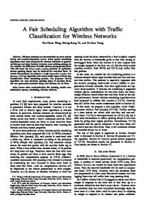
Figure 1: The proposed scheduling algorithm.

or asynchronous VCs will be selected to occupy this time slot according to the scheduling mechanism; if there are no valid frames in all VCs, an idle frame is generated and transmitted. During the asynchronous time slots, the virtual channels are scheduled with an algorithm based on VC urgency and frame urgency. Simulation results show that the proposed algorithm produces much less scheduling delay and higher channel utilization ratio than the DSA algorithm.

2. Scheduling Algorithm with Broad Applicability Based on Movable Boundary There are three kinds of virtual channels multiplexing modes [12]: the full synchronous multiplexing mode, the full asynchronous multiplexing mode, and the synchronous/ asynchronous multiplexing mode. For the full synchronous multiplexing mode, the order of virtual channels occupying

Mathematical Problems in Engineering

3

Begin

Are all asynchronous VCs empty?

Yes

Transmitting an idle frame

No Calculating the urgent degree function of each VC.

Is there only one VC with the largest value of Ui (k)?

Yes

Scheduling this VC

No Is there only one VC with the largest value of Ui (k) and pi ?

Yes

Scheduling this VC

No Scheduling the VC with the smallest serial number among them

The next scheduling time point

Figure 2: Asynchronous VCs scheduling algorithm.

a physical channel is fixed and repetitive, so it is suitable for the case in which most business data are synchronous and data rates of all the VCs are equivalent. However, it is not suitable for handling burst business and cannot achieve high channel utilization ratio. For the full asynchronous multiplexing mode, when two or more virtual channels are waiting to be scheduled, they are scheduled according to the priority assigned or calculated; therefore, this mode is suitable for burst business and low data rate information. However, this mode usually results in the delay wobbling of synchronous data [12]. For the synchronous/asynchronous multiplexing mode, the virtual channels are divided into synchronous and asynchronous ones. Synchronous virtual channels are scheduled with the full synchronous multiplexing mode, while asynchronous virtual channels are scheduled with the full asynchronous multiplexing mode. Although the system complexity is increased in this mode, the shortcomings of the first two modes mentioned above can be avoided. In order to reduce the scheduling delay and improve the channel utilization ratio, a virtual channels scheduling algorithm based on movable boundary is proposed. In the proposed algorithm, the synchronous/asynchronous

multiplexing mode is adopted. Time slots are divided into synchronous and asynchronous ones, which are used to schedule synchronous and asynchronous virtual channels, respectively. The system distributes the number of synchronous and asynchronous time slots according to the VC data rates and the number of VCs [12]. In terms of the scheduling strategy, the polling scheduling strategy is used for synchronous virtual channels, while the virtual channel scheduling strategy based on VC urgency and frame urgency is used for asynchronous virtual channels. The flowchart of the proposed scheduling algorithm is shown in Figure 1. 2.1. Synchronous Virtual Channel Scheduling Algorithm. For synchronous virtual channels, the polling scheduling algorithm is used. The so-called polling scheduling algorithm is that each virtual channel occupies the physical channel exactly according to the order assigned before. If there are no valid frames in the corresponding VC at a certain synchronous time point, the frame with the longest waiting time from the other synchronous VCs will be transmitted; if two or more frames from the other synchronous VCs have

4

Mathematical Problems in Engineering ×10−3 2.5

1 2.4

Average time delay of VC6 (s)

2.5 7 ×10 Downlink rate (bit/s) −4 ×10 2.8 Average time delay of VC5 (s)

2.45

2.6 2.4 2.2 2 1.8 2.4

2.45

2.5 7 ×10 Downlink rate (bit/s) 𝛽novel = 0.1 𝛽SAUB = 0.1 𝛽novel = 0.5 𝛽SAUB = 0.5 𝛽novel = 0.98 𝛽SAUB = 0.98 DSA

1.5 1 0.5 0 2.4

2.45

2.5 7 ×10 Downlink rate (bit/s)


2

2

1.5

1

0.5

0

2.4

2.45


×10−3 1.6

×10−4 2.8 2.6 2.4 2.2 2 1.8 2.4

2.45


1.5

1.4

1.3

1.2 2.4

1.5

1

0.5

0 2.4

2.45


×10−3 3 Average time delay of VC8 (s)

3


4

×10−3 2

×10−3 2




×10−3 5

2.45


2.5 2 1.5 1 0.5 2.4

2.45


Figure 3: The average time delay of each VC of source model 1.

the longest waiting time, the first frame in the synchronous VC with the smallest VC serial number among them is transmitted; if there are no valid frames in all synchronous VCs, a valid asynchronous frame will be selected and transmitted according to the asynchronous scheduling mechanism. Otherwise, an idle frame will be generated and transmitted through the physical channel. Define the waiting time of the current first frame in the ith VC (VC𝑖 ), 𝑇𝑤𝑖 , as: 𝑇𝑤𝑖 = 𝑘Δ𝑡 − 𝑇𝑖𝑎

𝑘 = 1, 2, 3, . . . ,

(1)

where 𝑘Δ𝑡 is the current scheduling time point, and 𝑇𝑖𝑎 is the arrival time of the current first frame in VC𝑖 . 2.2. Asynchronous Virtual Channel Scheduling Algorithm. For asynchronous virtual channels, the scheduling algorithm based on VC urgency and frame urgency is exploited. First, the VC urgency and frame urgency are calculated, respectively, and then they are balanced with a weighting coefficient

𝛽 to form a new urgent degree function of VCs. VCs are scheduled according to the values of the function. 2.2.1. VC Urgency. Define the transmission urgency of VC𝑖 , 𝑈1𝑖 (𝑘), as 𝑈1𝑖 (𝑘) = 𝑎𝑖 (𝑘) ⋅ 𝑄𝑖 (𝑘) ⋅ 𝑝𝑖 ,

(2)

where 𝑎𝑖 (𝑘) is the Boolean function, and it decides whether VC𝑖 can participate in the competition of the physical channel. The values of 𝑎𝑖 (𝑘) are shown as 1, { { { { 𝑎𝑖 (𝑘) = { { 0, { { {

there are some valid frames in VC𝑖 at the current scheduling time point there are no valid frames in VC𝑖 at the current scheduling time point.

(3)


6

2.5 ×107 Downlink rate (bit/s)

2.45


6.5 6 5.5 5 4.5

5

4

4 2.4

2.45 2.5 ×107 Downlink rate (bit/s) 𝛽novel = 0.1 𝛽SAUB = 0.1 𝛽novel = 0.5 𝛽SAUB = 0.5 𝛽novel = 0.98 𝛽SAUB = 0.98 DSA

3 2 1


2.4

2.45 2.5 ×107 Downlink rate (bit/s) 𝛽novel = 0.1 𝛽SAUB = 0.1 𝛽novel = 0.5 𝛽SAUB = 0.5 𝛽novel = 0.98 𝛽SAUB = 0.98 DSA

2.9 2.8 2.7 2.6

×10−3 5

4

3

2

1 2.4

2.45

×10−3 3

×10−4 Maximum time delay of VC6 (s)

Maximum time delay of VC5 (s)

2.4

4

0 2.4

0

2.45

×10−4 7

2


4 2.4

4


8

6

×10−3 5


10

×10−3 8




×10−3 12

5

2.45 2.5 ×107 Downlink rate (bit/s)

×10−3 5

2.5 2.4 2.45 2.5 ×107 Downlink rate (bit/s) 𝛽novel = 0.1 𝛽SAUB = 0.1 𝛽novel = 0.5 𝛽SAUB = 0.5 𝛽novel = 0.98 𝛽SAUB = 0.98 DSA

4

3

2

1 2.4 2.45 2.5 ×107 Downlink rate (bit/s) 𝛽novel = 0.1 𝛽SAUB = 0.1 𝛽novel = 0.5 𝛽SAUB = 0.5 𝛽novel = 0.98 𝛽SAUB = 0.98 DSA

Figure 4: The maximum time delay of each VC of source model 1.

𝑄𝑖 (𝑘) is the urgency base of VC𝑖 , and it calculates the delay from the last time point when VC𝑖 is scheduled to the current time point. The values of 𝑄𝑖 (𝑘) are shown as 𝑄𝑖 (𝑘) 0, { { { { { { { { { { { { { {𝑄 (𝑘 − 1) , ={ 𝑖 { { { { { { { { { { 𝑄 (𝑘 − 1) + 1, { { { 𝑖 {

2.2.2. Frame Urgency. Frame urgency can be calculated by the time that the current first frame has been waiting for. Define the frame urgency 𝑈2𝑖 (𝑘) of VC𝑖 as 𝑈2𝑖 (𝑘) = 𝑎𝑖 (𝑘) ⋅

there are some valid frames in VC𝑖 and VC𝑖 is scheduled at the 𝑘 − 1 time point there are some valid frames in VC𝑖 and VC𝑖 is not scheduled at the 𝑘 − 1 time point there are no valid frames in VC𝑖 at the 𝑘 − 1 time point. (4)

𝑝𝑖 is the static priority of VC𝑖 . If VC𝑖 requests higher real-time performance, a larger value of 𝑝𝑖 is assigned to it; otherwise, a smaller one is assigned.

(𝑘Δ𝑡 − 𝑇𝑖𝑎 ) ⋅ 𝑝𝑖 , Δ𝑡

(5)

where 𝑇𝑖𝑎 is the arrival time of the current first frame in VC𝑖 . Obviously, the smaller the value of 𝑇𝑖𝑎 is, the longer the waiting time of the current first frame is, which results in a larger value of 𝑈2𝑖 (𝑘). 2.2.3. Urgent Degree Function of Virtual Channel. Define the urgent degree function of VC𝑖 at the kth scheduling time point as 𝑈𝑖 (𝑘) = 𝛽 ⋅ 𝑈1𝑖 (𝑘) + (1 − 𝛽) ⋅ 𝑈2𝑖 (𝑘) , where 𝛽 is the weighting coefficient, 0 < 𝛽 < 1.

(6)

6


10

Maximum time delay of the system (s)

Channel utilization ratio

×10−3 12

−0.02

10−0.03 2.4

2.41 2.42 2.43 2.44 2.45 2.46 2.47 2.48 2.49 2.5 ×107 Downlink rate (bit/s) 𝛽novel = 0.1 𝛽SAUB = 0.1 𝛽novel = 0.5 𝛽SAUB = 0.5

11 10 9 8 7 6 5 4 2.4

2.41 2.42 2.43 2.44 2.45 2.46 2.47 2.48 2.49 Downlink rate (bit/s)

𝛽novel = 0.98 𝛽SAUB = 0.98 DSA

𝛽novel = 0.1 𝛽SAUB = 0.1 𝛽novel = 0.5 𝛽SAUB = 0.5

2.5 ×107


Figure 5: The channel utilization ratio of source model 1. Figure 7: The maximum time delay of system of source model 1.

Average time delay of the system (s)

×10−3 3.5 3 2.5 2 1.5 1 2.4

2.41 2.42 2.43 2.44 2.45 2.46 2.47 2.48 2.49 Downlink rate (bit/s) 𝛽novel = 0.1 𝛽SAUB = 0.1 𝛽novel = 0.5 𝛽SAUB = 0.5

2.5 ×107


Figure 6: The average time delay of system of source model 1.

frames in a VC are reset when the first frame in this VC is transmitted, which will result in the decline of the VC urgency. At any asynchronous scheduling time point, the VC with the largest value of 𝑈𝑖 (𝑘) is scheduled; if there are two or more VCs with the largest value of 𝑈𝑖 (𝑘), the VC with the largest values of 𝑈𝑖 (𝑘) and p𝑖 is scheduled; if there are two or more VCs with the largest values of 𝑈𝑖 (𝑘) and 𝑝𝑖 , the VC with the smallest VC serial number among them is scheduled. Otherwise, an idle frame is generated and transmitted through the physical channel. The flowchart of asynchronous VCs scheduling algorithm is shown in Figure 2. 2.2.4. Strategy of Selecting Weighting Coefficient. For different types of satellite data sources, we can select an appropriate 𝛽 by computer simulation to get good urgent degree functions of VCs so as to achieve good scheduling performance. Therefore, the proposed algorithm can be applied to diverse satellite data sources. Consider the following three kinds of satellite data sources.

Substituting (5) into (6), we can get 𝑈𝑖 (𝑘) = 𝑎𝑖 (𝑘) ⋅ [𝛽 ⋅ 𝑄𝑖 (𝑘) +

(1 − 𝛽) ⋅ (𝑘Δ𝑡 − 𝑇𝑖𝑎 ) ] ⋅ 𝑝𝑖 . Δ𝑡

(7)

As is shown in (7), both the VC urgency and the frame urgency are estimated when calculating the urgent degree functions of VCs. On one hand, this will prevent the VC with large amount of data from monopolizing the physical channel; on the other hand, it overcomes the problem in the literature [11–14] that the waiting time of the other data

(a) Sources with large difference among VC loads. For this kind of sources, there is usually one or more VCs with large amount of data, whose number of data frames is much larger than the others. For VCs with large amount of data, the values of frame urgency are relatively large and the values of VC urgency are relatively small at most scheduling time points; for VCs with little amount of data, whose time of occupying physical channel is limited, the values of VC urgency are relatively large and the values of frame urgency are relatively small at most scheduling time points. In order to prevent VCs with large amount of


3

2.95



×10−4

2

1

0 2.85

3

2.9

2.95

3 ×108 Downlink rate (bit/s) 𝛽novel = 0.1 𝛽SAUB = 0.1 𝛽novel = 0.5 𝛽SAUB = 0.5 𝛽novel = 0.98 𝛽SAUB = 0.98 DSA

6

4

2

0 2.85

2.9

2

1

0 2.85 2.9 2.95 3 ×108 Downlink rate (bit/s)


3 ×108 Downlink rate (bit/s) 2.9

4


2 2.85

5


4

6

2.95


6 5 4 3 2 2.85 2.9 2.95 3 ×108 Downlink rate (bit/s) ×10−4 3.5

0.012 Average time delay of VC8 (s)

5

×10−5 7

×10−4 Average time delay of VC3 (s)



×10−5 6

7

0.01 0.008 0.006 0.004 0.002 0 2.85

2.9

2.95


3 2.5 2 1.5 1 0.5 2.85

2.9 2.95 3 ×108 Downlink rate (bit/s) 𝛽novel = 0.1 𝛽SAUB = 0.1 𝛽novel = 0.5 𝛽SAUB = 0.5 𝛽novel = 0.98 𝛽SAUB = 0.98 DSA


data from monopolizing the physical channel, we can select large values for 𝛽.

3. Simulation Results

(b) Sources with moderate difference among VC loads. For this kind of sources, there are no VCs with enough data to monopolize physical channel, so the value of 𝛽 should be smaller than that of the first kind of sources. For the VCs with high data rates, the data frame urgency is dominant, so the smaller the value of 𝛽 is, the better the delay performance is; for the VCs with low data rates, the VC urgency is dominant, so the larger the value of 𝛽 is, the better the delay performance is. The right value of 𝛽 can be determined by VC loads and real-time requirements.

Simulation is performed to compare the performance of the novel algorithm we proposed with those of the SAUB algorithm and the DSA algorithm. It is worth mentioning that the SAUB algorithm is the algorithm in which the same scheduling strategies as those used in the proposed algorithm are adopted, except that the boundary between the synchronous time slots and asynchronous ones is unmovable. Performance parameters include mainly the average scheduling delay of each VC, the maximum scheduling delay of each VC, the average scheduling delay of system, and the maximum scheduling delay of system and the channel utilization ratio.

(c) Sources with little difference among VC loads. For this kind of sources, data rates of various VCs are relatively equivalent. Neither the VC urgency nor the frame urgency is dominant in the urgent degree function of VC, so the value of 𝛽 has little effect on the performance of VCs scheduling delay, which makes it easy to be selected.

3.1. Simulation on Sources with Large Difference among VC Loads. For this kind of sources, a source is selected whose VCs’ division and parameter settings are shown in Table 1. VC1∼VC6 are asynchronous VCs as that in the literature [15]. VC7 and VC8 are synchronous VCs. In addition, VC9 is used to generate and transmit idle frames. The highest data rate


1.1 1 0.9 2.85

2.9

3 ×108 Downlink rate (bit/s)

0.8 0.6 0.4 0.2 0 2.85

3 ×108 Downlink rate (bit/s) 2.9

3 2 2.9

2.95




1

4

1 2.85

2.95

×10−3 1.2

5

2.95

×10−3 2.5 2 1.5 1 0.5 0 2.85

2.9

2.95


𝛽novel = 0.1 𝛽SAUB = 0.1 𝛽novel = 0.5 𝛽SAUB = 0.5 𝛽novel = 0.98 𝛽SAUB = 0.98 DSA


1.2

6

×10−4 8

6

4

2

0.025 0.02 0.015 0.01 0.005 0 2.85



2.9

2.95

×10−4 1.6 1.4 1.2 1 0.8 0.6 2.85


3 2.9 2.95 ×108 Downlink rate (bit/s)


1.3


1.4

×10−4 7


×10−4 1.5



8

×10−4 7 6 5 4 3 2 2.85

2.9 2.95 3 ×108 Downlink rate (bit/s)



Figure 9: The maximum time delay of each VC of source model 2. Table 1: Source with large difference among VC loads. VC1 Type of source

High data rate source

Type of Path service service Data rate 15 (Mbps)

VC2

VC3

VC4


Middle data rate source


Path service

Path service

Path service

1.3

0.1

1.5

(VC1) is 300 times as large as the lowest data rate (VC6). The other simulation parameters are set as follows: (1) the length of data frame is 6000 bits; (2) downlink rate ranges from 2.4 × 107 bps to 2.5 × 107 bps; (3) the static priority values of VCs are 𝑝1 = 1.1, 𝑝2 = 1.2, 𝑝3 = 1.3, 𝑝4 = 1.4, 𝑝5 = 1.5, and 𝑝6 = 1.6, respectively. Simulation results are shown in Figures 3, 4, 5, 6, and 7. It is shown from the previous figures that for all the VCs, performance of the scheduling delay and the channel

VC5

VC6

VC7

Middle-low Low data rate High data data rate source rate source source Multiplexing Path service Path service service 0.06

0.05

3.3

VC8

VC9


Idle frame

Path service

—

1.1

—

utilization ratio achieved by the proposed algorithm are better than those achieved by the SAUB algorithm, no matter what the value of 𝛽 is. For example, when the downlink rate is 2.46 Mbps and 𝛽 is 0.98, the average scheduling delay of VC3, the maximum scheduling delay of VC3, and the channel utilization ratio achieved by the SAUB algorithm are 2.093 × 10−4 s, 8.671 × 10−4 s, and 0.9432, respectively, while those achieved by the proposed algorithm are 1.983×10−4 s, 8.485× 10−4 s, 0.9447, respectively. Therefore, the average scheduling

9




10−0.01

10−0.02

2.85

2.9

2.95

Downlink rate (bit/s) 𝛽novel = 0.1 𝛽SAUB = 0.1 𝛽novel = 0.5 𝛽SAUB = 0.5

3 ×108


10−3

2.85

2.9

2.95


Figure 10: The channel utilization ratio of source model 2.

Average time delay of the system (s)

10−2

3 ×108


Figure 12: The maximum time delay of system of source model 2.

the proposed algorithm are 25.56% and 15.25% lower than those achieved by the DSA algorithm, respectively, and the channel utilization ratio achieved by the proposed algorithm is 0.05% higher than that achieved by the DSA algorithm. When the value of 𝛽 is small, the performance of the proposed algorithm declines. This is consistent with our theoretical analysis. For all the VCs, scheduling delay varies with the change of 𝛽. In practice, we can select an appropriate value of 𝛽 to meet the delay requirements of all VCs without increasing the downlink rate. Obviously, such an advantage cannot be achieved by the DSA algorithm.

10−3

10−4 2.85

2.9

2.95

Downlink Rate(bit/s) 𝛽novel = 0.1 𝛽SAUB = 0.1 𝛽novel = 0.5 𝛽SAUB = 0.5

3 ×108



delay and the maximum scheduling delay of VC3 achieved by the proposed algorithm are 5.26% and 2.15% lower than those achieved by the SAUB algorithm, respectively, and the channel utilization ratio achieved by the proposed algorithm is 0.15% higher than that achieved by the SAUB algorithm. It is also shown that for most of the VCs, when the value of 𝛽 is large, performance achieved by the proposed algorithm is better than that achieved by the DSA algorithm. For example, when the downlink rate is 2.46 Mbps and 𝛽 is 0.98, the average scheduling delay of VC3, the maximum scheduling delay of VC3, and the channel utilization ratio achieved by the DSA algorithm are 2.664 × 10−4 s, 1.001 × 10−3 s, and 0.9442, respectively. Therefore, the average scheduling delay and the maximum scheduling delay of VC3 achieved by

3.2. Simulation on Sources with Moderate Difference among VC Loads. For this kind of sources, manned spacecraft source model [16] is used, whose VCs’ division and parameter settings are shown in Table 2. VC1∼VC6 are asynchronous VCs. VC7 and VC8 are synchronous VCs. In addition, VC9 is used to generate and transmit idle frames. The highest data rate (VC6) is 47.5 times as large as the lowest data rate (VC4). The other simulation parameters are set as follows: (1) the length of data frame is 8000 bits; (2) downlink rate ranges from 2.85 × 108 bps to 3.0 × 108 bps; (3) the static priority values of VCs are 𝑝1 = 1.6, 𝑝2 = 1.5, 𝑝3 = 1.4, 𝑝4 = 1.3, 𝑝5 = 1.2, and 𝑝6 = 1.1, respectively. Simulation results are shown in Figures 8, 9, 10, 11, and 12. Similar to model 1, for most of the VCs, the performance of the proposed algorithm is better than that of the SAUB algorithm and that of the DSA algorithm, no matter what the value of 𝛽 is. For example, when the downlink rate is 2.91 Mbps and 𝛽 is 0.5, the average scheduling delay of VC3, the maximum scheduling delay of VC3, and the channel utilization ratio achieved by the SAUB algorithm are 1.123 × 10−4 s, 4.358 × 10−4 s, and 0.9691, respectively, those achieved by the DSA algorithm are 1.339 × 10−4 s, 6.734 × 10−4 s, and 0.9680, respectively, and those achieved by the proposed

10


1.65




×10−3 3

2 1.5 1 0.5 0 1.6

1.65

2 1.5 1 0.5

1.7


7 6 5 4 3 2 1

0 1.6 1.65 1.7 1.75 8 Downlink rate (bit/s) ×10



2.5

0 1.6 1.65 1.7 1.75 8 ×10 Downlink rate (bit/s) −4 ×10 8

1.7

2.5

3

0.8 0.6 0.4 0.2 0 1.6 1.65 1.7 1.75 8 Downlink rate (bit/s) ×10 ×10−4 2.35 2.3 2.25 2.2 2.15 2.1 2.05 1.6

1.7

6 5 4 3 2 1 1.6

×10−4 3.2

1.75 8 Downlink rate (bit/s) ×10


1.65

7

0


0 1.6


0.5

3.5


1

×10−4 8

×10−3 1



×10−3 1.5

1.65 1.7 1.75 8 Downlink rate (bit/s) ×10

3 2.8 2.6 2.4 2.2 1.6

1.75 8 Downlink rate (bit/s) ×10


1.65

1.7



Table 2: Manned spacecraft source model.

Type of source Type of service Data rate (Mbps)

VC1

VC2

VC3

VC4

VC5

VC6

Platform network data

Physiological telemetry data

Delayed telemetry data

Internet data

Test data

CCD image data

Path service

Path service

Path service

Internet service

Path service

10

10

35

2

75

algorithm are 9.287 × 10−5 s, 3.459 × 10−4 s, and 0.9692, respectively. Therefore, compared with those achieved by the SAUB algorithm, the average scheduling delay and the maximum scheduling delay of VC3 achieved by the proposed algorithm are 17.30% and 20.63% lower, respectively, and the channel utilization ratio achieved by the proposed algorithm

VC7

VC8

Bit-stream service

Video surveillance data Bit-stream service

Video conference data Bit-stream service

95

44

11

VC9 Idle frame — —

is 0.01% higher; compared with those achieved by the DSA algorithm, the average scheduling delay and the maximum scheduling delay of VC3 achieved by the proposed algorithm are 30.64% and 48.63% lower, respectively, and the channel utilization ratio achieved by the proposed algorithm is 0.12% higher.

2 1

0.008 0.006 0.004 0.002 0 1.6

1.7

1.65

0.006 0.004 0.002

0 1.6 1.65 1.7 1.75 8 Downlink rate (bit/s) ×10 𝛽novel = 0.1 𝛽SAUB = 0.1 𝛽novel = 0.5 𝛽SAUB = 0.5 𝛽novel = 0.98 𝛽SAUB = 0.98 DSA

1.5

1

0.5

0 1.6

0.5

1.65

1.75 1.65 1.7 8 Downlink rate (bit/s) ×10 𝛽novel = 0.1 𝛽SAUB = 0.1 𝛽novel = 0.5 𝛽SAUB = 0.5 𝛽novel = 0.98 𝛽SAUB = 0.98 DSA

1.5 1 0.5

1.65

1.7

1.75 ×108

Downlink rate (bit/s) ×10−4 6.5

4.75 4.7 4.65 4.6 4.55 4.5 4.45 4.4 1.6

2

0 1.6

1.7

×10−4 4.8 Maximum time delay of VC7 (s)


0.008

1


1.7

×10−3 2

0.01

1.5

0 1.6




1.65

0.01


3


4

×10−3 2.5

×10−3 2

0.012

5

0 1.6

11


×10−3 6 Maximum time delay of VC2 (s)



1.75 8 Downlink rate (bit/s)×10 1.65

1.7


6

5.5

5

4.5 1.6

1.65 1.7 1.75 8 Downlink rate (bit/s)×10 𝛽novel = 0.1 𝛽SAUB = 0.1 𝛽novel = 0.5 𝛽SAUB = 0.5 𝛽novel = 0.98 𝛽SAUB = 0.98 DSA

Figure 14: The maximum time delay of each VC of source model 3.

For the VCs with high data rates (e.g., VC6), the smaller the value of 𝛽 is, the shorter the scheduling delay is; for the VCs with lower data rates (e.g., VC3), the larger the value of 𝛽 is, the shorter the scheduling delay is, which is consistent with theoretical analysis.

3.3. Simulation on Sources with Little Difference among VC Loads. For this kind of sources, a source is selected whose VCs’ division and parameter settings are shown in Table 3. VC1∼VC6 are asynchronous VCs as shown in the literature [17]. VC7 and VC8 are synchronous VCs. In addition, VC9 is used to generate and transmit idle frames. In order to make the experimental results reflect balanced loads in general sense, the data rates of VC1–VC8 are set around 20 Mbps, but they are slightly different. The other simulation parameters are set as follows: (1) the data frame length is 6000 bits; (2) downlink rate ranges from 1.6 × 108 bps to 1.75 × 108 bps;

(3) the static priority values of VCs are 𝑝1 = 1.1, 𝑝2 = 1.2, 𝑝3 = 1.3, 𝑝4 = 1.4, 𝑝5 = 1.5, and 𝑝6 = 1.6, respectively. Simulation results are shown in Figures 13, 14, 15, 16, and 17. Similar to source model 1 and model 2, for most of the VCs, the performance of the proposed algorithm is better than that of the SAUB algorithm and the DSA algorithm, no matter what the value of 𝛽 is. For example, when the downlink rate is 1.63 Mbps and 𝛽 is 0.1, the average scheduling delay of VC3, the maximum scheduling delay of VC3, and the channel utilization ratio achieved by the SAUB algorithm are 4.882 × 10−4 s, 1.978 × 10−3 s, and 0.9833, respectively; those achieved by the DSA algorithm are 8.443 × 10−4 s, 5.943 × 10−3 s, and 0.9827, respectively, and those achieved by the proposed algorithm are 4.204 × 10−4 s, 1.889 × 10−3 , and 0.9833, respectively. Therefore, compared with those achieved by the SAUB algorithm, the average scheduling delay and the maximum scheduling delay of VC3 achieved by the

12

Mathematical Problems in Engineering Table 3: Source with little difference among VC loads. VC1

VC2

Type of High data High data source rate source rate source Type of Path service Path service service Data rate 20 21 (Mbps)

VC3

VC4

VC5

VC6

VC7

VC8

VC9







Idle frame

Path service

Path service

Path service

Path service

Path service

Path service

—

19.5

19

22

18.5

19

21

—


1


0.99 0.98 0.97 0.96 0.95 0.94 0.93

10−2

10−3

0.92 1.6

1.65

1.7


1.75 ×108

1.65

1.7



Figure 15: The channel utilization ratio of source model 3.

1.75 ×108


Figure 17: The maximum time delay of system of source model 3.

proposed algorithm are 13.89% and 4.50% lower, respectively; compared with those achieved by the DSA algorithm, the average scheduling delay and the maximum scheduling delay of VC3 achieved by the proposed algorithm are 50.21% and 68.21% lower, respectively, and the channel utilization ratio achieved by the proposed algorithm is 0.06% higher. Because data rates of all the VCs are equivalent, the value of 𝛽 has relatively little effect on the performance of scheduling delay.

×10−3 1.4 Average time delay of the system (s)

1.6

1.2 1 0.8 0.6

4. Conclusions

0.4 0.2 0 1.6

1.65

1.7


1.75 ×108



We proposed a novel algorithm for virtual channel scheduling based on movable boundary, in which time slots are divided into synchronous ones and asynchronous ones. During the synchronous time slots, the polling scheduling algorithm is used, while during the asynchronous ones, the VC scheduling algorithm based on VC urgency and frame urgency is used. When there are no valid synchronous data frames in the corresponding VC at a certain synchronous time slot, a frame of the other synchronous VC or asynchronous VCs will be transmitted. If there are no valid frames in all VCs, an idle frame will be generated and transmitted. Compared with

Mathematical Problems in Engineering the SAUB algorithm, the proposed algorithm can reduce the scheduling delay and improve the channel utilization ratio, while compared with the DSA algorithm, the proposed algorithm is much better as far as the time delay and applicability scope are concerned. In addition, the proposed algorithm is suitable for the scheduling of diverse data sources.

Acknowledgments This work was supported by the Natural Science Foundation of China (61101116), the Outstanding Young Scholar Plan of Liaoning Province (LJQ2012018), the Innovative Team Project of Liaoning (LT2011T005), and the Open Foundation of Key Laboratory of Shenyang Ligong University (4771004kfs06).

References [1] Space Packet Protocol, Recommendation For Space Data System Standards, CCSDS 133.0-B-1, Blue Book, Issue 1, CCSDS, Washington, DC, USA, 2003. [2] Overview of Space Link Protocols, Consultative Committee For Space Data System. CCSDS 130. 0-G-1, Draft Green Book, CCSDS, 2004. [3] AOS space data link protocol, Recommendation For Space Data System Standards, CCSDS 732.0-B-1, Blue Book, Issue 1, CCSDS, Washington, DC, USA, 2003. [4] AOS space data link protocol, Recommendation For Space Data System Standards, CCSDS 732.0-B-2, Blue Book, Issue 2, CCSDS, Washington, DC, USA, 2006. [5] Y. Tian, X. Na, Y. Xia, X.-L. Gao, and L.-S. Liu, “Research on the performance and application of adaptive frame generation algorithm in AOS protocol,” Journal of Astronautics, vol. 33, no. 2, pp. 242–248, 2012. [6] Y. Tian, C.-S. Pan, Z.-J. Zhang, and Y.-Q. Zhang, “Research on adaptive frame generation algorithm in AOS protocol,” Journal of Astronautics, vol. 32, no. 5, pp. 1171–1178, 2011. [7] Y. Tian, D. Zhang, Z. Tan, C. Pan, and X. Gao, “Research on the packet time delay of frame generation algorithms in advanced orbiting systems,” Chinese High Technology Letters, vol. 21, no. 11, pp. 1121–1128, 2011. [8] Y.-T. Zhao, C.-S. Pan, Y. Tian, Z.-J. Zhang, and M.-X. Bi, “Research on multiplexing efficiency of MPDU based on CCSDS advanced orbiting systems,” Journal of Astronautics, vol. 31, no. 4, pp. 1195–1199, 2010. [9] Y. Wen, Study of Advanced Orbiting System Multiplexer, Inner Mongolia University of Technology, Hohhot, China, 2007. [10] Y. Q. Gu and W. Z. Tan, “CCSDS downlink virtual channel schedule and performance analysis,” Chinese Space Science and Technology, vol. 21, pp. 29–35, 2001. [11] A. P. Riha and C. Okino, “An advanced orbiting systems approach to quality of service in space-based intelligent communication networks,” in Proceedings of the 27th IEEE Aerospace Conference, Big Sky, March 2006. [12] Y.-X. Bie, C.-S. Pan, and R.-Y. Cai, “Research and simulation on AOS virtual channel multiplexing technique,” Journal of Astronautics, vol. 32, no. 1, pp. 193–198, 2011. [13] G. Z. Shao, Z. B. Hua, J. J. Sun et al., “Design and Implementation of On-board Packard Telemetry Equipment,” Journal of Telemetry, Tracking, and Command, vol. 22, pp. 9–14, 2001.

13 [14] Q. Liu, C. Pan, G. Wang, and W. Liu, “CCSDS advanced orbiting systems, data links protocol: Study on virtual channels scheduling algorithm,” in Proceedings of the 8th International Conference on Intelligent Systems Design and Applications (ISDA ’08), pp. 351–355, November 2008. [15] Y. K. Ma, Z. Z. Zhang, and N. T. Zhang, “Simulation study on data processing system based on CCSDS AOS,” Journal of Telemetry, Tracking , and Command, vol. 23, pp. 26–30, 2002. [16] Z. Tian and Q. J. Zhang, “Research on advanced orbiting systems virtual channels scheduling sstrategy of manned spacecraft,” Spacecraft Engineering, vol. 15, pp. 20–26, 2006. [17] Y. Zhao, High Data Rate Multi-Connect Encoder, Xidian University, Xi’an, China, 2007.

Advances in

Operations Research Hindawi Publishing Corporation http://www.hindawi.com

Volume 2014

Advances in

Decision Sciences Hindawi Publishing Corporation http://www.hindawi.com

Volume 2014

Journal of

Applied Mathematics

Algebra

Hindawi Publishing Corporation http://www.hindawi.com


Volume 2014

Journal of

Probability and Statistics Volume 2014

The Scientific World Journal Hindawi Publishing Corporation http://www.hindawi.com


Volume 2014

International Journal of

Differential Equations Hindawi Publishing Corporation http://www.hindawi.com

Volume 2014

Volume 2014

Submit your manuscripts at http://www.hindawi.com International Journal of

Advances in

Combinatorics Hindawi Publishing Corporation http://www.hindawi.com

Mathematical Physics Hindawi Publishing Corporation http://www.hindawi.com

Volume 2014

Journal of

Complex Analysis Hindawi Publishing Corporation http://www.hindawi.com

Volume 2014

International Journal of Mathematics and Mathematical Sciences


Journal of

Mathematics Hindawi Publishing Corporation http://www.hindawi.com

Volume 2014


Volume 2014

Volume 2014


Volume 2014

Discrete Mathematics

Journal of

Volume 2014


Discrete Dynamics in Nature and Society

Journal of

Function Spaces Hindawi Publishing Corporation http://www.hindawi.com

Abstract and Applied Analysis

Volume 2014


Volume 2014


Volume 2014

International Journal of

Journal of

Stochastic Analysis

Optimization



Volume 2014

Volume 2014