reducing the learning curve of knee arthroscopy interventions, we have developed a training system for virtual arthroscopic knee surgery. We adopt the Visible ...
A Virtual Reality Training System for Knee Arthroscopic Surgery Pheng-Ann Heng, Chun-Yiu Cheng, Tien-Tsin Wong, Yangsheng Xu, Yim-Pan Chui, Kai-Ming Chan, Shiu-Kit Tso
Abstract— Surgical training systems based on virtual-reality (VR) simulation techniques offer a cost-effective and efficient alternative to traditional training methods. This paper describes a VR system for training arthroscopic knee surgery. Virtual models used in this system are constructed from the Visual Human Project dataset. Our system simulates soft tissue deformation with topological change in real-time using finite element analysis. To offer realistic tactile feedback, we build a tailor-made force feedback hardware.
I. I NTRODUCTION In last two decades, minimally invasive micro-surgical techniques have revolutionized the practice of surgery in orthopedics, otolaryngology, gastroenterology, gynecology and abdominal surgeries. Compared to conventional open surgery, minimally invasive surgery (MIS), or namely, endoscopic surgery, offers less trauma, reduced pain and quicker patient convalescence. However, in endoscopic surgery, the restricted vision, non-intuitive hand-eye coordination and limited mobility of surgical instruments can easily cause unexpected injuries to patients. Excellent skill of hand-eye co-ordination and accurate instrumental manipulation are essential for surgeons to perform MIS safely. Extensive training of novice medical officers and interns to master the skill of endoscopic surgery is one of the major issues in MIS practice. Currently, the most common method for surgical training is to use animals, cadavers or plastic models. However, the anatomy of animals differs from that of humans. Cadavers cannot be used repeatedly while their tactile feeling is much different from that of living body. Training with plastic model cannot provide realistic visual and haptic feedback. VR Simulation systems provide an elegant solution to these problems, because we can create virtual models of different anatomic structures and use them to simulate different procedures within the virtual environment. A VR-based system can be reused many times and a systematic education training programme can be fully integrated with the VR-based system without risking patient’s health. As a solution that helps reducing the learning curve of knee arthroscopy interventions, we have developed a training system for virtual arthroscopic knee surgery. We adopt the Visible Human Project dataset [1] to construct the virtual models. The real-time deformation and cutting of soft tissue with topological change is simulated using finite element analysis (FEA). To deliver tactile realism, we build a tailor-made force feedback hardware device. The details of our system will be discussed in later sections.
II. R ELATED W ORK A great deal of research effort has been directed toward developing MIS systems in the recent years. Some recent simulation systems for laparoscopic surgery and arthroscopic surgery have been presented in [2] [3] [4], but these systems are not tailored for knee surgery. The knee arthroscopic surgery systems presented in [5] [6] mostly rely on highend workstations for real-time visualization. Some of these simulators still lack force feedback and cannot demonstrate real-time topological changes of anatomic structures. Virtual models in these systems are relatively simple and not realistic enough. The system KATS [7] adopts a mock-up leg and sensors to simulate the virtual knee arthroscopic surgery. Though visual feedback is achieved, only limited haptic feedback is provided by the mock-up leg model. The system enables good cognitive learning module, however, structural anatomic deformation is not modeled.
(a)
(b)
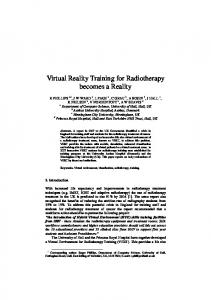
Fig. 1. Illustration of forces imposed by PHANToM Desktop, the arrows show the direction of the imposed force. (a) A 3-DOF positional force can be imposed by the device. (b) The torque feedback cannot be imposed.
The system VR-AKS [8] has been developed by the American Academy of Orthopaedic Surgeons (AAOS). Their system adopts a volumetric representation for anatomic structure and uses the PHANToM Desktop [9] as the haptic feedback interface. However, due to the hardware limitation of the PHANToM Desktop, the system can only impose positional force (see Fig. 1(a)) on the tip of stylus, while in a realistically simulated system, torque feedback (Fig. 1(b)) should also be imposed on the tip of the stylus. III. U SER I NTERFACE To overcome the haptic insufficiency of existing hardwares, we develope a force feedback device which can satisfy the simulation requirement. Our device presents more realistic forces, including both kinds of forces illustrated in Fig. 1 to users. This enables the trainee surgeon to be engaged within
the virtual environment in a more realistic manner, so that the haptic perception of different tissues can be improved. To achieve real-time anatomic deformation and cutting, we propose a hybrid finite element method (FEM) to simulate soft tissue topological change.
(a)
(b)
(c)
(d)
(e)
(f)
Fig. 2. Comparison of real arthroscopic surgery with our VR-based surgery system. (a) Real interface for the knee arthroscopic surgery. (d) Virtual twohand haptic input interface. (b) & (c) Real screen shots from the knee arthroscope. (e) & (f) Simulated views.
A complete surgical simulator should allow the trainee surgeon to perform a standard inspection. Our system presents a two-hand arthroscope-like interface (Fig. 2(d)). Users can manipulate a virtual arthroscope or probe with haptic feedback. A real arthroscope provides a 30 degree adjustable offset viewing at its tip; our system allows the user to adjust this rotation by rotating the knob at the tip of our arthroscope. The field-of-view is also adjustable.
arthroscope camera 30°
(a)
(b)
The meniscus and the probe are shown. The views from our simulated virtual arthroscopic surgery are shown in Fig. 2(e) & (f) for comparison. Our two-hand haptic device (Fig. 3(a)) provides a 4-DOF motion mechanism for each handle. The first three DOFs (with force feedback): pitch (Fig. 3(c)), yaw (Fig. 3(d)) and insertion (Fig. 3(e)), enable the arthroscope or instrument to move in a way similar to a real arthroscope. The fourth rotational DOF (without force feedback) enables surgeons to look around the immediate vicinity of the 30-degree arthroscope tip (Fig. 3(b)). The position and the orientation of tips of arthroscope/surgical instruments are tracked by three optical encoders, while force feedback is driven by three DC servo motors.
(a)
(b)
(c) arthroscope
arthroscope
arthroscope
probe
probe
probe
(d)
(e)
(f)
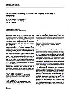
Fig. 4. (a), (b) & (c) Different internal views of the virtual endoscope (d), (e) & (f) Corresponding external views of the knee. From left to right, the leg is bent.
Fig. 4 shows different rendered views of our virtual knee arthroscopy. Fig. 4(a), (b) & (c) show the internal structure observed through the virtual arthroscope, while Fig. 4(d), (e) & (f) illustrate the corresponding external views. In this example, the left tool mimics the arthroscope while the right tool mimics the probe. From the image on the left of Fig. 4 to those on the right, flexion of the knee joint increases. With different bending postures of the leg, the surgeon can diagnose different parts of the knee joint. In Fig. 4(c), we can clearly observe the meniscus and ligament of the virtual knee. IV. S YSTEM A RCHITECTURE
(c)
(d)
(e)
Fig. 3. The tailor-made haptics device (a) Outlook of the bare device. (b) The 30 degree bending at the tip of the arthroscope. The degree of freedom in our haptic device. (c) Pitch, (d) Yaw, and (e) Insertion.
Our system supports inspection training, such as recognizing major landmarks at the knee joint and navigating the compartments of knee through the virtual arthroscope. Fig. 2(b) & (c) are screen shots captured from a real knee arthroscope.
The hardware of our system is composed of an input-andoutput haptic device, a PC, and a display screen. The haptic device gives the user not only 4-DOF navigating parameters (pitch, yaw, insertion and camera rotation), but also force feedback when there is a collision or when operating on soft tissues. Our system is executed on a Pentium IV 1.5GHz PC equipped with nVidia GeForce3 graphics board. The PC handles all computation including FEA, collision detection and realistic rendering. Fig. 5 shows the software architecture of our system. We adopt OpenGL and C++ to develop our software. The overall system flow consists a pre-processing phase and a run-time phase. In preprocessing phase, knee-joint compartments are
Preprocessing phase CT, MRI Volume Data
Segmented Volume Data
Segmentation
Run-time phase
Surface and Tetrahedral mesh
Tool Positional Data
Force Feedback Device
Visual Rendering
Fig. 5.
Haptic Rendering parameters
tetrahedral mesh for deformable model (e.g ligament)
Surface and Tetrahedral Mesh Generation
2D slices
-Collision Detection -Real-time Soft tissue deformation -Force feedback calculation of soft tissue
Surface mesh
Surface mesh
Simplify & Smooth
combined model
Tetrahedral mesh
Local Remesh in Operational region
surface mesh for non-deformable model (e.g. bone)
The system architecture of the virtual arthroscopy training system.
modelled. Both surface models and tetrahedral models are generated for FEA computation. Runtime operations includes collision detection, soft tissue deformation and cutting, local remeshing, realistic rendering and the communication with the embedded micro-controller in the haptic device. The microcontroller tracks the position and orientation of two handles and drives the haptic device to feed back force based on the result of soft tissue deformation. The preprocessing phase is discussed in Section V. In Section VI, we discuss the real-time soft tissue deformation, where our proposed hybrid FE model is illustrated. In Section VII, the soft tissue cutting algorithm and the tetrahedral mesh simplification are presented. Section VIII outlines the process of collision detection. Section IX describes the haptic interface and results. V. S EGMENTATION AND M ESH G ENERATION A. Segmentation and Surface Mesh Generation In our system, two types of meshes are generated. We model the non-deformable organs, such as bone, using surface meshes. On the other hand, we generate tetrahedral meshes to represent deformable organs, such as muscle and ligament. These two mesh generation steps are performed in the preprocessing phase (Fig. 5). We used slices no. 2131-2310 from the Visible Human Project image dataset to segment the organs of interest from these slices. A semi-automatic seed-based method is used to obtain a 2D contour from each slice. Our method is a modified snake segmentation. From the result of segmentation on a series of CT or MRI images, we obtain a volume in which we tag the tissue (organ) type of each voxel. Surface mesh is created from the series of 2D contours using the 3D reconstruction algorithm. We use the method proposed by Ganapathy [10] to construct the surface mesh. Since each contour of a single slice can be identified by its two neighboring tissues, there is no correspondence problem in our case. Fig. 6 outlines the overall procedure in generating meshes. B. Constrained Tetrahedral Mesh Generation There are two major methods to create the tetrahedral mesh from a segmented volume. Interval volume tetrahedraliza-
(a)
(b)
Fig. 6. (a) The generation of both surface meshes (for non-deformable structures) and tetrahedral meshes (for deformable structures) from the slices of medical images. (b) The resultant meshes for bone and muscular structures.
tion [11] tessellates the generated interval volume. Because the size of a tetrahedron is smaller than a voxel, the generated mesh usually contains too many tetrahedra, and thus making the real-time FEA difficult. Another method [12] tetrahedralizes isosurfaces using the 3D Delaunay tetrahedralization algorithm. The advantage of this method is that it preserves the detail boundary of different organs/structures. In other words, Delaunay triangulation guarantees the final mesh to be wellshaped. However, when two organs/structures are adjacent, the algorithm may mistakenly introduce gaps between the two generated meshes. To solve these problems, we have previously proposed a constrained tetrahedral mesh generation algorithm [13] for extracting human organs from the segmented volume. Our method is an incremental insertion algorithm in Delaunay triangulation category, which creates the tetrahedral mesh directly from the segmented volume with no need in generating isosurfaces in advance. Our method can preserve as much geometric details as the algorithm presented in [12], while at the same time our generated tetrahedral mesh can be kept small-scaled and wellshaped for posterior FEA computation. The mesh generation process can be fully automatic or provide a flexibility of adjusting the mesh resolution. The whole algorithm consists of two main phases: �
Vertex Placement This phase is mainly responsible for placing vertices to facilitate the subsequent tetrahedralization. It affects the mesh density and conformation to tissue boundaries. Section V-C describes the details. � Boundary-Preserved Delaunay Tetrahedralization Without additional constraints, preservation of boundary positions between different structures may not be guaranteed during the tetrahedralization. We combine an incremental insertion method and a flipping-based algorithm to generate tetrahedral meshes. Three remeshing operations are carried out succeedingly in order to restore tissue boundaries. We discuss the tetrahedralization in Section V-D.
C. Vertex Placement There are two kinds of vertices, namely, feature points and Steiner points. Feature points are points on the surface of the organ, which represent the geometrical structure of organ. The placement of feature points affects the mesh conformation to the organ boundary. Steiner points are the interior points within the surface boundary of the organ. The placement of Steiner points affects the mesh density. To avoid unexpected gaps between different meshes, we apply a discrete structure in our vertex model. The placement of all vertices are based on this structure. 1) Feature Point Selection: Feature points are of abrupt gradient change in the local neighborhood. For simplicity, we place the feature points at the mid-points of voxel edges (edges connecting two adjacent voxel samples). Fig. 7 denotes the possible positions of feature points, in which the grid points of the lattice are voxel samples. Placement of feature points undergoes three steps: � gradient computation at every mid-point of the voxel edge � gradient comparison in the local neighborhood � error-bounded reduction of feature points Gradient is computed at every mid-point of the voxel edge. There are three types of mid-points, x+0.5, y+0.5 and z +0.5, which lie on the voxel edges aligned to x, y and z axes, respectively. We compute the gradient of midpoint by linearly interpolating gradients of two ending voxels. The gradient of this midpoint is then compared with that of its 8 neighbors (black nodes in Fig. 7) on x plane (Fig. 7(a)), y plane (Fig. 7(b)), and z plane (Fig. 7(c)). If the gradient difference exceeds a user-defined threshold, this mid-point is selected as a feature point.
mesh quality, we insert Steiner points (interior points). To do so, we define a density field D(x� y� z ). For any point (x� y� z ) in the volume, we obtain a field value:
D(x� y� z ) =
n X k
=1
�Dk
Q
�
d x� y� z ) k =1 = d x� y� z )
Pn
=
j6 k j ( Qn j6 k j (
(1)
where n is the total number of feature points; Subscript k denotes a feature point; Dk is the distance from the k-th feature point to the closest feature point; � is a user-defined constant which controls the mesh density; dk (x� y� z ) is the distance between the input point (x� y� z ) to the k-th feature point (x k � yk � zk ). For each voxel sample position, we compute the field value D(x� y� z ). Then we go through each of them and compare its field value D with all other D values within the local neighborhood of radius r. If the current voxel position holds a field value with a local absolute difference larger than a predefined threshold, it is selected as a Steiner point. D. Boundary-Preserved Delaunay Tetrahedralization 1) Boundary Preservation: Unless additional constraints are imposed, the tetrahedral mesh generated by 3D Delaunay tetrahedralization may not preserve organ boundaries. Fig. 8(a) illustrates an example where the dashed line is a boundary. We apply a remeshing algorithm to restore the boundary. Fig. 8(b) shows the result after restoring the boundary.
Fig. 8. (a) Before remeshing for boundary preservation. (b) After remeshing. (c) The boundary-preserved tetrahedral mesh.
(a)
(b)
(c)
Fig. 7. The gradient of an interested mid-point (the white node) is compared with its neighboring mid-points (black nodes) for feature point detection. (a) x+0.5 neighbors (b) y+0.5 neighbors (c) z+0.5 neighbors.
However, this results in enormous feature points. Hence we perform a of this midpoint simplification by merging feature points. Here, we define a global error limit to reduce feature points in the local neighborhood. We merge two feature points if their gradient difference is less than a global error bound. To merge the feature points, we randomly select one of them for replacement. In addition, if two feature points are on edges which share a common vertex, or the tissue types of the two ends of both feature points are the same, they can also be merged. 2) Steiner Point Insertion: With these feature points, we can obtain a coarse tetrahedral mesh by 3D Delaunay tetrahedralization. However, the quality of this coarse tetrahedral mesh is not satisfactory for FEM computation. To improve the
If a boundary-crossing is detected, the remeshing algorithm is applied to ensure all tetrahedra follow the boundary constraint. Our remeshing algorithm is a flip-based tetrahedralization method. It takes the following three major steps: � finding all the tetrahedra containing the crossing edge � finding the remaining faces and points to form new tetrahedra � tessellating and constructing new faces and tetrahedra We propose three primitive flip operations: flip23, flip32, and flip4diagonal (Fig. 9).
Fig. 9.
Primitive flip operations to restore the boundary.
2) Tissue Type Tagging: After remeshing, we tag each tetrahedron to indicate its tissue type. If the tetrahedron encloses any voxel sample position, we can simply assign the tissue type of the enclosed voxel sample to this tetrahedron. Otherwise, trilinear interpolation is used to lookup the tissue type at the centroid of the tetrahedron. Fig. 10 shows the tagged tetrahedron meshes.
Different tissues exhibit different stiffness features. We adopt tissue physical properties from [16] to compute different stiffness matrix for each tissue. operational region
shared node non-operational region
Fig. 11.
The hybrid model.
The equations of linear system for the operational and nonoperational regions are formulated as a form of block matrices: (a)
(b)
(c)
�
Fig. 10. Tagged tetrahedral meshes, (a) fat-muscle-bone (b) muscle-bone, and (c) bone.
The adaptive mesh generated is accurate and well-shaped so that it is suitable for 3D finite element solvers. As an example, for a segmented volume with resolution of 297 � 341 � 180, our algorithm generates a tetrahedral mesh of 94,953 vertices and 490,409 tetrahedra. VI. S OFT T ISSUE D EFORMATION Previous works on soft tissue deformation has not simultaneously achieved both the realism of expensive physical simulation and real-time interaction. Finite element models are suitable for computing accurate and complex deformation of soft tissues in surgery simulation [14]. However, it is impossible to achieve real-time deformation unless a certain degree of simplification is applied. It is necessary to provide the ability to cut and suture the tissue in addition to tissue deformation. To simulate the tissue cutting and suturing, finite element models need remeshing, followed by re-computation of the stiffness matrix (also known as load vector in standard FEM literatures). The intensive computation makes it extremely difficult to achieve real-time performance. To achieve real-time feedback, we have proposed a deformation model, called hybrid condensed FE model [15], based on the volumetric finite element method. The hybrid FE model consists of two regions, an operational region and a non-operational one (Fig. 11). During the surgical operation, most operations are conducted on a local pathological area of the organ. Hence, we model the pathological area as the operational region. We assume that topological change occurs only in the operational region throughout surgery. Different models are designed to treat regions with different properties in order to balance the computation time and the level of simulation realism. We use a complex FE model, which can deal with non-linear deformation and topological change, to model the small-scale operational region. Conversely, we use a linear and topology-fixed FE model, in which the generation speed can be accelerated by pre-computation, to model the large-scale non-operational region. Since these two regions are connected to each other through shared vertices, additional boundary conditions have to be introduced to both models.
�
��
Kpp Kpc Kcp Kcc Kcc Kcn Knc Knn
�
Ap Ac
��
� =
Ac An
�
Pp Pc
�
Pc Pn
�
2
Pc Ps Pi
(2)
;
� =
(3)
where K is the stiffness matrix; A is the displacement vector; Subscripts p and n represent the operational and nonoperational regions respectively; Subscript c represents the common vertices shared by these two regions; Pc and ;Pc are the force and counterforce respectively applied to the common vertices when we analyze these two regions. The interior vertices of the non-operational region are irrelevant to any action of the surgeon, and may be regarded as redundant vertices during simulation. To speed up calculation, a condensation process [17] is applied to remove those vertices from the non-operational region for computation. As a result, the dimension of matrices computed during FEA is reduced, which in turn speeds up the computation. To show how the force computation within the nonoperational region can be sped up after condensation, we rewrite the equation for non-operational region in the condensed form:
2 4
Kcc Kcs Kci Ksc Kss Ksi Kic Kis Kii
32 54
3
Ac As Ai
5
=
4
3 5
(4)
where Pc is the mutual force applied to the shared vertices when we analyze these two regions respectively. The subscripts c, i and s represent the shared vertices between operational and non-operational regions, the interior vertices and the retained surface vertices, respectively. Deduced from Equation (4), we obtain a new matrix equation which only relates to the variables of the surface vertices:
K � As = P �
(5)
where
Kss Ksi Kii;1 Kis and ;1 = Ps + (Ksi Kii Kic Ksc ) Ac It should be noted that the form of P � has one term, Ac , that relates to the shared vertices. In other words, after solving Ac , we can obtain P � at once and so forth the displacement vector. K� P�
=
;
�
�
�
�
;
�
VII. C UTTING
AND
M ESH S IMPLIFICATION
B. Cutting the Tetrahedral Mesh
Soft tissue cutting is supported within the operational region. We present a new cutting algorithm for this soft tissue simulation. Firstly, we subdivide tetrahedra by tracking the actual intersection points between the cutting tool and each tetrahedron. Then we generate cut surfaces between these intersection points. Fig. 12 shows a simple example of the cutting.
When a tetrahedron is cut, five general cases can be identified after considering rotation and symmetry (Fig. 14). The first case is when 3 edges are cut and a tip of the tetrahedron is separated from the rest of the tetrahedron. The second case shows 4 edges are cut, and the tetrahedron is evenly split into two. The third case shows a partially cut tetrahedron, where 2 faces and an edge are intersected. The last two cases show another two types of partially cut tetrahedron.
Fig. 12.
Fig. 14.
Example of tissue cutting.
Our algorithm [18] works on tetrahedral meshes. It uses the minimal new element creation method [19], which generates as few new tetrahedra as possible after each cut. Progressive cutting with temporary subdivision is adopted both to give the user interactive visual feedback and to constrain the number of new tetrahedra to an acceptable level.
Five general cases of tetrahedron subdivision.
1) Crack-free Tetrahedral Subdivision: For a tetrahedral subdivision to be crack-free, the subdivision on adjacent faces must be consistent [20]. There are, in total, eight kinds of subdivision in the algorithm, which are demonstrated in Fig. 15.
A. General Cutting Procedure The major steps in our cutting algorithm are shown in Fig. 13. Firstly, the initial intersection between the cutting tool and the model is detected. We determine if the cutting tool moves across any of the surface boundaries. Once an intersection is detected, we record the intersected tetrahedron in which the initial intersection test occurs. For all tetrahedron faces and edges that are intersected, we propagate the intersection test to neighboring tetrahedra that share the faces or edges. This allows us to quickly detect the involved tetrahedra. Then, for each tetrahedron that has been intersected, we subdivide the tetrahedron once the cut is completed. Process start Collision detection between motion of cutter and surface triangle, initials the list of intersected tetrahedrons
Yes
Optimize the new mesh; generate the new initial list of intersected tetrahedrons, then wait for use input
Yes
Is the initial list of intersected tetrahedrons empty?
No
No
For each intersected tetrahedron, judge if the edges and faces is cut. Then subdivide it
Fig. 13.
General procedure for cutting.
Is the list of intersected tetrahedrons empty?
If the face of the tetrahedron is cut, then add the neighbor tetrahedrons to the list
Fig. 15.
Eight kinds of subdivision of faces.
2) Progressive Cutting: Since users always expect an immediate visual feedback during the cutting progress, updating virtual models is required while cutting. We update the tetrahedron subdivision at certain time intervals. Each subdivision update is based on the cutting result of the previous time instance. Fig. 16 shows the rendered frames. However, the number of tetrahedra will increase very quickly as the user cuts. As Fig. 16 shows, the number of tetrahedra increases from 1 to 20 after three updates. Another way of progressive cutting is to subdivide a tetrahedron temporarily until it is completely cut. The temporarily subdivided tetrahedron is discarded after display. Fig. 17 shows the subdivision when this approach is used. When the cutting tool moves and if the topology of the subdivided tetrahedron doesn’t change, only the position of the intersection points has to be updated. If the topology changes, the temporary tetrahedra are deleted and the tetrahedron is resubdivided. With this approach, the total number of tetrahedra will increase moderately. The latency between user input and visual feedback can be reduced.
2) Vertex Replacement: Edge collapse may change the position of a vertex on the surface which in turn influences the mesh quality. As a common rule, if one end of the collapsing edge is on the surface and the other is interior, the new vertex after edge collapse should be set at the position of the one on the surface. Otherwise, the new vertex will be set at the mid-point of the edge.
Fig. 16.
Subdivision based on previous step.
Fig. 19.
Fig. 17.
Subdivision based on the original untouched tetrahedron.
C. Tetrahedral Mesh Simplification After cutting, the cut mesh may contain many tiny long triangles (Fig. 18(a)). To improve the mesh quality and speed up later computation, we perform a mesh simplification. Fig. 18(b) shows the result after mesh simplification. Mesh simplification is focused on the newly created tetrahedra, not on the whole tetrahedral mesh. Therefore, most of the original tetrahedra which are far away from the cutting region remain unchanged during the simplification. Only a few tetrahedra near the cutting region are affected. The simplification method is as follows:
(a)
(b)
Fig. 18. (a) Cutting result without mesh simplification. (b) Cutting result with mesh simplification.
1) Edge Selection: The primitive operation for simplification is edge collapse. For each edge collapse operation, an edge is selected. There are many ways for selecting a proper edge, such as the shortest edge in meshes, the shortest edge in the smallest triangle, or the shortest edge in the smallest tetrahedron. Since it is expensive to search for the optimal one, an edge is selected from the interested tetrahedron based on a greedy method.
Example of inversion due to edge collapse.
3) Inversion Detection: During edge collapse, tetrahedra sharing two vertices will be affected. Their vertices will be replaced by the merged vertex. However, unexpected inversion may occur during this replacement. Hence, before the collapse, each affected tetrahedron must be checked for the possibility of inversion. If inversion is detected, the collapse should be rejected. In Fig. 19, e(V1 , V2 ) is the edge to collapse and the new vertex v is set to be V2 . If the collapse is performed, tetrahedron t(V1 � V3 � V4� V5) will become t(v� V3 � V4� V5). Vertices v and V1 will be on opposite side of face f (V3 � V4� V5) and tetrahedron t(V1 � V3 � V4� V5) is inversed.
(a) Fig. 20.
(b)
Two types of undesired topological change due to edge collapse.
4) Topological Change Detection: Edge collapse may also introduce two types of unexpected topological changes (Fig. 20) which should be avoided. Suppose that e(V1 � V2) is the edge to be collapsed. In Fig. 20 (a), V1 and V2 are both vertices on the surface, and edge e(V1 � V2) is also an edge on the surface, and there is a triangular hole besides edge e(V1 � V2). If the collapse is performed, the hole will disappear. In Fig. 20(b), edge e(V1 � V2) is an edge on the surface, but there is a surface three-point loop v V1 V2 . If edge collapse is performed, parts A and B will be connected by an edge instead of a face.
Fig. 21.
Distance from the new vertex v .
5) Boundary Error Computation: Vertices on the surface may be shifted after edge collapse, this may change the appearance of mesh. To maintain the shape, edge collapse is controlled using a boundary error threshold. If, after collapse, the maximum distance between the new vertex, v, and the original surface exceeds the threshold, the collapse should be rejected. To speed up checking, we simply bound the projected distance from v to its original triangle, as illustrated in Fig. 21. Because the adjacent new triangles on the cutting surface are almost coplanar, this simplification works well with a low boundary error threshold. 6) Edge Collapse: Once the selected edge passes all the above checks, edge collapse is performed. Given the collapsed edge e(V1 � V2), tetrahedra sharing e are deleted. Tetrahedra connected with either V1 or V2 are updated by replacing V1 or V2 with new vertex v. Edges ended with either V1 or V2 are updated by replacing its end with v. VIII. C OLLISION D ETECTION In our simulation system, collision detection is used in computing the interaction between arthroscope and organs during navigation and the interaction between scalpel and ligament during cutting. Traditional methods for collision detection are mostly designed for rigid objects: hierarchical bounding box structures are pre-computed as structures that do not change too much during the simulation. Unfortunately, most of these methods are not suitable for deformable objects. For deformable objects, bounding boxes have to be updated frequently during surface deformation and cutting. To update these bounding boxes, we adopt an axis-aligned bounding boxes (AABB) tree as the data structure for our collision detection algorithm. Like other collision detection methods, our AABB-tree is constructed from top to bottom. Firstly, the bounding box of the whole surface mesh is computed. Note that surface mesh alone (without the tetrahedral mesh) is sufficient for computing collision detection. The surface mesh is divided into two groups. For each group, its bounding boxes are constructed and inserted into the AABBtree. The subdivision is recursively performed until every leaf node contains only one triangle. During cutting, surface triangles are subdivided and new triangles are created. There are two types of new triangles, the first type is simply the subdivided triangles while the other is created along the cutting path. For the first type, we construct sub-trees, each contains triangles resulted from the subdivision of the original triangles. Then the parent triangle node is replaced with the sub-tree. For the second type, we construct a sub-tree to contain all newly generated triangles, and then insert it into the original tree at the corresponding position. For those leaf nodes containing triangles that are removed or degenerated, they can be removed from the AABB-tree. No matter how the AABB-tree is updated, the modified tree may become loose after several updates. Therefore, we should reconstruct a tighter AABB-tree when the system is idle. IX. R ESULTS Once the system starts, the application enters a continuous force feedback loop. The haptic device feeds the positional and
orientational input to the PC and the collision detection between virtual devices and organs is then computed according to this information. Corresponding tissue deformation is reflected while forces are calculated based on mass-spring model. Force output signal is delivered to the haptic device for final haptic rendering. The resultant input and output latency is less than 10ms. Throughout the whole system development process, medical professionals, including two of our authors, from the Department of Orthopaedics and Traumatology of the same university, are involved in commenting implementation details and evaluating the system. A satisfactory tactile feedback is achieved according to their expertise. With haptic rendering, surgeon trainee can inspect the internal structure with realistic tactile feeling and can differentiate different tissue types. Our system provides a “procedure recording” function so that the medical expertise’s manipulation of the virtual arthroscope and tool can be saved. Once the whole recording process is completed, we can play back the whole procedure and ask medical students to practice the same procedure repeatedly. Currently, our system is under a clinical testing stage where medical students are invited to evaluate our system and they do feel comfortable with our training interface. X. C ONCLUSION We have developed a virtual reality system for training knee arthroscopic surgery. Mesh generation, real-time soft tissue deformation, cutting and collision detection are presented to users. Realistic haptic rendering is provided by our system while real-time performance is achieved. Medical experts satisfy with the tactile feedback given by our system and find its application on training hand-eye coordination useful. In the future, we plan to develop a smaller portable version of the haptic device which offers even more realistic user interface. ACKNOWLEDGMENT The authors would like to thank G. Zhang, S. S. Zhao, Z. Tang, X. Yang, H. Shen and W. Guo for their contribution in this project. The work described in this paper was fully supported by a grant from the Research Grants Council of the Hong Kong Special Administrative Region. (Project no. CUHK1/00C). R EFERENCES [1] M. J. Ackerman, “The Visible Human Project,” in Proceedings of IEEE, 86(3), 504-11, 1998. [2] M. Downes, M. C. Cavusoglu, W. Gantert, L. W. Way, and F. Tendick, “Virtual Environment for Training Critical Skills in Laparoscopic Surgery,” in Proceedings of Medicine Meets Virtual Reality, pp. 316– 322, 1998. [3] “The Karlsruhe Endoscopic Surgery Trainer.” http://iregt1.iai.fzk.de/TRAINER/mic trainer1.html. [4] “ENT Surgical Simulator.” http://www.lockheedmartin.com/factsheets/product526.html. [5] S. Gibson, J. Samosky, A. Mor, C. Fyock, E. Grimson, T. Kanade, R. Kikinis, H. Lauer, N. McKenzie, S. Nakajima, H. Ohkami, R. Osborne, and A. Sawada, “Simulating Arthroscopic Knee Surgery Using Volumetric Object Representations, Real-time Volume Rendering and Haptic Feedback,” in Proceedings of First Joint Conference CVRMedMRCAS’97, pp. 369–378, 1997.
[6] A. D. McCarthy and R. J. Hollands, “A Commercially Viable Virtual Reality Knee Arthroscopy Training System,” in Proceedings of Medicine Meets Virtual Reality, pp. 302–308, 1998. [7] G. Megali, O. Tonet, M. Mazzoni, P. Dario, A. Vascellari, and M. Macacci, “A New Tool for Surgical Training in Knee Arthroscopy,” in Proceedings of the Medical Image Computing and Computer-Assisted Intervention, Pt. 2. 2002, Lecture Notes in Computer Science, Vol. 2489, (Tokyo, Japan), pp. 170–177, Springer, September 2002. [8] J. D. Mabrey, S. D. Gilogly, J. R. Kasser, H. J. Sweeney, B. Zarins, H. Mevis, W. E. Garrett, R. Poss, and W. D. Cannon, “Virtual Reality Simulation of Arthroscopy of the Knee,” The Journal of Arthroscopic and Related Surgery, vol. 18, July-August 2002. [9] T. H. Massie and J. K. Salisbury, “The PHANTOM Haptic Interface: A Device for Probing Virtual Objects,” in Proceedings of the ASME Winter Annual Meeting, Symposium on Haptic Interfaces for Virtual Environment and Teleoperator Systems, 1994. [10] S. Ganapathy and T. G. Dennehy, “A new general triangulation method for planar contours,” Computer Graphics (Proceedings of SIGGRAPH), vol. 16, no. 3, pp. 69–75, 1982. [11] G. M. Nielson and J. Sung, “Interval volume tetrahedralization,” in Visualization’97, pp. 221–228, 1997. [12] J. M. Sullivan, J. Z. Wu, and A. Kulkarni, “Three-dimensional finiteelement mesh generation of anatomically accurate organs using surface geometries created from the visible human dataset,” in Proceedings of The Third Visible Human Project Conference, October 2000. [13] X. Yang, P. A. Heng, and Z. Tang, “Constrained Tetrahedral Mesh Generation of Human Organs on Segmented Volume,” in Proceedings of International Conference on Diagnostic Imaging and Analysis, (Shanghai, China), pp. 294–299, August 2002. [14] H. Delingette, “Towards realistic soft tissue modeling in medical simulation,” in Proceedings of the IEEE: Special Issue on Surgery Simulation, pp. 521–523, April 1998. [15] W. Wu, J. Sun, and P. A. Heng, “A Hybrid Condensed Finite Element Model for Interactive 3D Soft Tissue Cutting,” in Proceedings of The Eleventh Annual Medicine Meets Virtual Reality Conference (MMVR11), January 2003. [16] F. A. Duck, Physical Properties of Tissue - A Comprehensive Reference Book. Academic Press, 1990. [17] M. Bro-Nielsen and S. Cotin, “Real-Time Volumetric Deformable Models for Surgery Simulation Using Finite Elements and Condensation,” in Proceedings of Eurographics’96 - Computer Graphics Forum, vol. 15, pp. 57–66, 1996. [18] J. Sun, W. Guo, J. Chai, and Z. Tang, “Simulation of surgery cutting,” in In Proceedings of the Fourth China-Japan-Korea Joint Symposium on Medical Informatics, July 2002. [19] A. B. Mor and T. Kanade, “Modify soft tissue models: Progressive cutting with minimal new element creation,” in Proceedings of the Medical Image Computing and Computer-Assisted Intervention, pp. 598–607, 2000. [20] H. W. Nienhuys and A. F. van der Stappen, “Supporting cuts and finite element deformation in interactive surgery simulation,” tech. rep., Institute of Information and Computing Science, Utrecht University, 2001.