A Warm Rain Microphysics Parameterization that Includes the Effect of ...

JUNE 2008

FRANKLIN

1795

A Warm Rain Microphysics Parameterization that Includes the Effect of Turbulence CHARMAINE N. FRANKLIN Centre for Australian Weather and Climate Research,* Melbourne, Victoria, Australia (Manuscript received 28 June 2007, in final form 30 October 2007) ABSTRACT A warm rain parameterization has been developed by solving the stochastic collection equation with the use of turbulent collision kernels. The resulting parameterizations for the processes of autoconversion, accretion, and self-collection are functions of the turbulent intensity of the flow and are applicable to turbulent cloud conditions ranging in dissipation rates of turbulent kinetic energy from 100 to 1500 cm2 s⫺3. Turbulence has a significant effect on the acceleration of the drop size distribution and can reduce the time to the formation of raindrops. When the stochastic collection equation is solved with the gravitational collision kernel for an initial distribution with a liquid water content of 1 g m⫺3 and 240 drops cm⫺3 with a mean volume radius of 10 ␮m, the amount of mass that is transferred to drop sizes greater than 40 ␮m in radius after 20 min is 0.9% of the total mass. When the stochastic collection equation is solved with a turbulent collision kernel for collector drops in the range of 10–30 ␮m with a dissipation rate of turbulent kinetic energy equal to 100 cm2 s⫺3, this percentage increases to 21.4. Increasing the dissipation rate of turbulent kinetic energy to 500, 1000, and 1500 cm2 s⫺3 further increases the percentage of mass transferred to radii greater than 40 ␮m after 20 min to 41%, 52%, and 58%, respectively, showing a substantial acceleration of the drop size distribution when a turbulent collision kernel that includes both turbulent and gravitational forcing replaces the purely gravitational kernel. The warm rain microphysics parameterization has been developed from direct numerical simulation (DNS) results that are characterized by Reynolds numbers that are orders of magnitude smaller than those of atmospheric turbulence. The uncertainty involved with the extrapolation of the results to high Reynolds numbers, the use of gravitational collision efficiencies, and the range of the droplets for which the effect of turbulence has been included should all be considered when interpreting results based on these new microphysics parameterizations.

1. Introduction The representation of cloud microphysical properties is a crucial component of atmospheric models. The effect of aerosols on clouds remains one of the largest sources of uncertainty in climate studies and many of the complex aerosol–cloud interactions are associated with cloud microphysical processes (Beard and Ochs 1993). To enable greater confidence in climate projections one of the processes that requires a quantitative analysis is the second indirect aerosol effect, which is the effect from enhanced aerosol concentrations in

* The Centre for Australian Weather and Climate Research is a partnership between the Australian Bureau of Meteorology and CSIRO, Melbourne, Victoria, Australia.

Corresponding author address: Dr. Charmaine Franklin, CSIRO Marine and Atmospheric Research, Private Bag No. 1, Aspendale, VIC 3195, Australia. E-mail: [email protected] DOI: 10.1175/2007JAS2556.1 © 2008 American Meteorological Society

clouds suppressing drizzle and prolonging cloud lifetimes (Albrecht 1989). To be able to quantify this effect with any real certainty, the cloud microphysical processes must be accurately represented in global climate models (GCMs), in particular the autoconversion process, which describes the collision and coalescence of small cloud droplets to form larger raindrops. Rotstayn and Liu (2005) demonstrated how changing autoconversion schemes in a GCM could decrease the globally averaged second indirect aerosol effect by 60%, highlighting the need for increased understanding and a more accurate parameterization of autoconversion. In addition to the importance of microphysics in GCMs, high-resolution numerical weather prediction models require detailed representations of cloud microphysics to produce accurate quantitative precipitation forecasts (e.g., Fritsch and Carbone 2004). In clouds where the temperature does not reach freezing, cloud droplets initially grow through the process of condensation. The rate of increase of drop radius caused by condensation growth decreases with in-

1796

JOURNAL OF THE ATMOSPHERIC SCIENCES

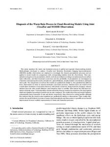
FIG. 1. Schematic diagram of the competing effects of condensation and collision–coalescence growth of cloud droplets as a function of time.

creasing radius, and it is the process of collision and coalescence that allows drops to grow to a size large enough to fall out of a cloud as rain (see Fig. 1). When the equations governing these two modes of droplet growth are applied to describe observed warm cloud droplet growth times there is a discrepancy between the observed and theoretically calculated growth rates. Observations tend to show a faster evolution and broader drop size distribution (e.g., Beard and Ochs 1993) compared to the theoretically calculated drop spectra, where the equations are applied to a randomly distributed population of drops and their motion is only governed by gravitational forcing. Several physical effects have been suggested to play an important role in the reduction of the growth times, including entrainment and mixing of dry air, turbulence, and the role of giant cloud condensation nuclei (e.g., Beard and Ochs 1993; Jonas 1996; Shaw 2003). There are hints of turbulence increasing the collision rate of cloud droplets in some observational data. For example, the observations of Feingold et al. (1999) indicated that there was in general a positive correlation between in-cloud turbulence and radar reflectivity. This could simply be due to more vigorous clouds having greater cloud liquid water contents and/or due to the drops having a greater residence time in the cloud, allowing them to collide and coalesce with a larger number of droplets as suggested by Mason (1952) and described by a turbulent collision kernel. Turbulence increases the collision rate of droplets in at least three ways: by changing the droplet velocities and the spatial distribution of the droplets (e.g., Franklin et al. 2005) and by changing the collision and coalescence efficiencies between droplets. There has been some observational support for the clustering of cloud droplets in a turbulent flow as seen in direct numerical simulations (DNSs; Franklin et al. 2005, 2007; Wang et al.

VOLUME 65

2005). Pinsky and Khain (2003) observed clusters of droplets in cumulus clouds and Lehmann et al. (2007) showed that droplet clustering was evident in even weakly turbulent clouds. Although the effect of turbulence on cloud droplet collision–coalescence rates is yet to be quantified by observations, recent modeling studies have shown that turbulence can increase the collision rates of droplets by several times the purely gravitational rate (Wang et al. 2005; Pinsky et al. 2006; Franklin et al. 2007). Autoconversion is the process whereby small cloud droplets collide and coalesce to form larger raindrops. The ideal way to model autoconversion in numerical models is to use an explicit bin microphysics model, which minimizes the need to parameterize cloud microphysical processes. Unfortunately the computational cost of this approach is out of reach for most modeling applications and therefore the vast majority of atmospheric models must use parameterized cloud microphysics. Kessler (1969) first introduced the concept of representing microphysical processes by the separate cloud and rain liquid water contents. The separation of the drop size distribution into two populations stems from a bulk modeling requirement to treat separately the cloud drops with small terminal velocities that move with the airflow and the larger raindrops with appreciable terminal velocities that sediment through the cloud. Autoconversion parameterizations are derived either from analytical approximations of the collision kernel or from empirical fits to model data, where the data used are either a numerical solution of the stochastic collection equation (SCE) using an accurate collision kernel or a large eddy simulation (LES) model with explicit microphysics. The analytically derived schemes use fixed forms of the drop size distribution, which is a significant limitation because the functional forms of the drop size distribution change significantly in space and time in reality (e.g., Zawadzki et al. 1994). An additional limitation of the analytically based autoconversion parameterizations is the use of a simplified solution of the collision kernel because a complete analytical solution does not exist. Long’s (1974) kernel, which represents the collision kernel as a piecewise polynomial, has been used in autoconversion parameterizations derived by Manton and Cotton (1977), Seifert and Beheng (2001), and Liu et al. (2006) to name a few. Apart from the errors introduced in these forms of the autoconversion rate through the constant form of the drop size distribution, Long’s approximate kernel has been shown to give a faster evolution of the drop size distribution than the more accurate collision kernel composed by Hall (1980; see Feingold et al. 1997). Empirically based autoconversion parameterizations that

JUNE 2008

use numerical solutions of the exact form of the collision kernel can simulate a range of drop size distributions that are applicable to many cloud types and at various stages of a cloud’s lifetime. The model-based empirical parameterizations derive autoconversion rates as functions of bulk cloud properties. This approach has been used by Beheng (1994) and Khairoutdinov and Kogan (2000) and is the one adopted in this study. The next section introduces the methodology used in this work. Section 3 examines the effect of turbulence on the evolution of the drop size distribution. New warm rain parameterizations that include the effect of turbulence are derived in section 4, and section 5 includes a detailed comparison of the new autoconversion parameterization with other existing models. The results and their implications are discussed in section 6.

2. Methodology a. Turbulent collision kernel The geometric collision kernel is described by ⌫共r1 ⫹ r2兲 ⫽ 2␲共r1 ⫹ r2兲2具 | wr | 典g共r1 ⫹ r2兲 cm3s⫺1, 共1兲 where r1 and r2 are the radii of the interacting droplets, 具 | wr | 典 is the average of the absolute value of the radial relative velocities between the droplets, and g(r1 ⫹ r2) is the radial distribution function that measures the preferential concentration or clustering between the droplets from the two size groups. In the purely gravitational case the relative velocity is the difference between the terminal velocities of the droplets and there is no clustering, hence g(r1 ⫹ r2) ⫽ 1. When the droplet motion is a function of both gravitational and turbulent accelerations, the values of wr and g(r1 ⫹ r2) become much more complex and no analytical solution is available. Direct numerical simulations of the droplets within the turbulent flow field have been performed by Franklin et al. (2005, 2007) and the result of that work has been the development of empirically derived equations that describe the turbulent radial relative velocities and the clustering of drop pairs, with the larger droplet within the radius range of 10–30 ␮m and the eddy dissipation rate of turbulent kinetic energy of the flow between 100 and 1500 cm2 s⫺3. The parameterizations for these processes are (Franklin et al. 2007)

具 | wr | 典turb | wr | gravR␭

1797

FRANKLIN

0.0145

⫽ 0.0195

e

␷t1␷t2 ␷␩2

g共r1 ⫹ r2兲 共⫺0.3331兲 ⫽ ⫺0.0139 e R␭

⫹ 0.0084

and

共2兲

⫹ 0.0394,

共3兲

␷t1␷t2 ␷␩2

FIG. 2. Comparison of the parameterized turbulent collision kernel with the collision rate data directly from the DNS experiments.

where R␭ is the Taylor-based Reynolds number of the DNS flow, ␷t1 and ␷t2 are the terminal velocities of the drops, and ␷␩ is the Kolmogorov velocity, which is the characteristic velocity of the small-scale eddies of the flow. Together these equations give the turbulent geometric collision kernel (1), which is shown in Fig. 2 to be a good fit to the DNS data. The main criticism of DNS is the significantly lower Reynolds numbers of the simulated flow fields compared to atmospheric turbulence. DNS is limited in the range of scales that it can simulate because of computational requirements, and this limits the largest scales and consequently the Reynolds number of the flow. As discussed in detail in Franklin et al. (2007), there are uncertainties involved in extrapolating the collision rates over orders of magnitudes of Reynolds numbers, and whether the rates increase linearly, saturate, or exhibit some other form of behavior with increasing Reynolds number is unknown at this time. However, it needs to be emphasized here that because of the unknown effect of an increased Reynolds number on the DNS statistics, the results in this study should be interpreted with the necessary precautions. The parameterization of the turbulent collision kernel was developed from the DNS data, and, therefore, when using (2) and (3) a Reynolds number that is consistent with the DNS needs to be used. The following power law relates the Reynolds number from the simulations to the eddy dissipation rate of turbulent kinetic energy (TKE; Franklin et al. 2007), where ␧ has units of cm2 s⫺3: R␭ ⫽ 21␧0.12.

共4兲

As shown by Franklin et al. (2007) the turbulent parameterizations tend to underestimate the DNS data,

1798

JOURNAL OF THE ATMOSPHERIC SCIENCES

VOLUME 65

FIG. 3. Turbulent collision kernels normalized by the corresponding gravitational kernel for the eddy dissipation rates of (a) 100, (b) 500, (c) 1000, and (d) 1500 cm2 s⫺3. The lowest contour plotted is 1.1, i.e., the turbulent collision kernel is 10% greater than the gravitational kernel for these interacting droplet sizes, and the contour levels increase by 0.2. Note that the reason why the turbulent kernel is not equal to the gravitational kernel for drop sizes slightly greater than 30 ␮m is because the mean radius of the neighboring mass bins increases from 29.5 to 32.5, so the effects of the turbulence are felt through to the mean radius of 32.5. The regions along the diagonals are free from contours because in this region there is a discontinuity, as the gravitational kernel that is being used to normalize the turbulent kernel is equal to zero for equal-sized drops at these points.

particularly for the highest level of turbulence. This underestimation becomes apparent in the comparison of Fig. 3, which shows the turbulent collision kernels from the parameterizations normalized by the corresponding gravitational collision kernel, and Fig. 4 of Franklin et al. (2007), which shows the normalized kernels based on the DNS data. The parameterized kernel is a maximum of 2.7 times greater than the gravitational kernel for the highest dissipation rate and the 30-␮m collector drop (see Fig. 3), whereas the DNS data show a maximum increase of more than 8 times for this same case. There are also cases where the parameterized kernel overpredicts the DNS data; however, these differences are not as significant as the underpredictions. Therefore, compared to the DNS data, the results in this paper that use the parameterized kernel will tend to show a lesser impact of turbulence.

b. Stochastic collection equation The collision and coalescence of drops is described analytically by the SCE. This equation is given by Pruppacher and Klett (1997) as ⭸n共x, t兲 ⫽ ⭸t

冕

x1

n共xc,t兲K共xc,x⬘兲n共x⬘,t兲 dx⬘

x0

⫺

冕

⬁

n共x, t兲K共x, x⬘兲n共x⬘, t兲 dx⬘,

共5兲

x0

where n(x, t) is the drop number distribution function, x is the mass of the drop that is formed when the drops of mass xc and x⬘ collide and form a larger drop, K(xc, x⬘) is the collection kernel for drops sizes xc and x⬘ (which is the geometric collision kernel multiplied by the collision and coalescence efficiencies), x0 is the mass

JUNE 2008

FRANKLIN

of the smallest droplet, and x1 ⫽ x/2. The first integral represents the gain rate of drops of mass x through the collision and coalescence of two smaller drops xc and x⬘, while the second integral represents the loss of drops of mass x through these drops coalescing with other drops to form a larger-sized drop. The stochastic nature of the collision process comes into the equation through the collection kernel K, which is related to the probability that two drops of particular sizes will collide within a unit volume within a unit of time. In this study, Bott’s (1998) flux method is used to solve the SCE but with the exponential functions of Bott (2000) to describe the mass flux. This method is mass conservative, numerically efficient, and produces generally very good agreement with the Berry and Reinhardt scheme (1974), which is known to be highly accurate. A comprehensive analysis of the efficiency, stability, and accuracy of this scheme has been conducted by Bott (1998, 2000). The numerical solutions use a logarithmically equidistant mass grid, where the mass doubles after three grid cells and the time step used is 1 s. There are 160 bins with drop radii from 0.6 to 104 ␮m. Detailed numerical tests were undertaken to ensure the convergence and accuracy of the solution of the SCE. Decreasing the time step to 0.1 s results in a difference in the mean mass-weighted radius after 20 min of less than 0.07%, and increasing the bin resolution by a factor of 4 produces a difference in this radius of 1%. In the numerical experiments the hydrodynamic kernel of Hall (1980) is used where the terminal velocities are those of Beard (1977), the collision efficiencies come from a range of sources depending on the collector droplet size, and the coalescence efficiency is set to 1. To examine the effect of turbulence on the evolution of the drop size distribution through simulations of the SCE, the gravitational geometric collision kernel has been replaced by the turbulent kernel of Franklin et al. (2007) for collector drops in the radius range of 10–30 ␮m. For the range of turbulent flow parameters examined in this study, DNS data do not exist to describe droplet collision rates for the entire drop size distribution. The DNS experiments on which the turbulent collision kernel is based in Franklin et al. (2007) cover the range of drop sizes that are believed to be the most important for the process of rain initiation in warm clouds (see, e.g., Vaillancourt and Yau 2000; Pinsky and Khain 2004). Turbulence will have a smaller but nonzero effect on collision rates between droplets with a collector size a little smaller than 10 ␮m in radius and somewhat larger than 30 ␮m; however, at exactly what size the effects become negligible is unknown at this

1799

time for the range of turbulent flow parameters of interest. Unpublished DNS results by the author have confirmed the expectation that the effect of turbulence on droplets larger than 30 ␮m in radius will begin to diminish. These results show that the effect of turbulence on a droplet pair of 30 and 40 ␮m in radii is smaller than the effect on a droplet pair of 22.5 and 30 ␮m for all four dissipation rates of TKE studied in Franklin et al. (2007). This is due to droplets of these larger sizes having significant terminal velocities that dominate the motion of the droplet and restrict the time that the drops can interact with turbulent vortices, thus reducing the effect of turbulence. These four additional DNS experiments do not contain enough information to extend the parameterization of Franklin et al. (2007) beyond the largest collector drop size of 30 ␮m and as DNS are computationally very expensive, at this stage the range of validity of the turbulent collision kernel parameterization used in this study is 10–30 ␮m for the collector droplet radius. In the current study where a defined collision kernel for the entire drop size distribution is required, the choice had to be made to either 1) set the effect of turbulence to zero outside of the range of validity of the turbulent geometric collision kernel parameterization or 2) apply some function to the turbulent collision kernel parameterization for collector droplets smaller than 10 ␮m in radius and larger than 30 ␮m that decreases the effect of turbulence for some arbitrary range of droplet sizes outside of the range for which DNS data are available for the turbulent flow parameters of interest. In this study method 1) was chosen so that the results are an underestimate of the effect of turbulence rather than a potential overestimate. Neither approach is ideal; however, a choice of one or the other is necessary to evaluate the effect of turbulence on autoconversion given the state of the science at the present time. Once DNS data become available for more collector droplet sizes it may be necessary to reevaluate the effect of turbulence on the evolution of the drop size distribution and modify the coefficients of the warm rain microphysics parameterization; this should be considered when using the results of this study. For the autoconversion process, which is the most problematic warm rain process for the cloud physics community, extending the turbulent collision kernel parameterization will only change the results of this study if the effect of turbulence on collisions is significant for collector droplets in the radius range 30 ⬍ r ⬍ 40 ␮m, since the autoconversion process, as defined in this present study, does not consider collisions with a collector droplet having a radius larger than 40 ␮m (see section 4). In these experiments the gravitational colli-

1800

JOURNAL OF THE ATMOSPHERIC SCIENCES

VOLUME 65

FIG. 4. Temporal evolution of the mass-weighted mean radius for the gravitational and four turbulent cases for (a) the first 20 min of the simulation and (b) the full 60-min simulation. Each solution was obtained from the integration of the SCE where the LWC was 1 g m⫺3, the initial number concentration was 240 drops cm⫺3, the relative dispersion of the initial drop size distribution was 0.57, and the mean volume radius was 10 ␮m.

sion efficiency has been used for all collector drop sizes as the effect of turbulence on the collision efficiencies of small droplets is still unclear. An examination of the possible consequences of using the gravitational collision efficiency for the turbulent experiments is conducted in section 3b.

3. Effect of turbulence on the evolution of the drop size distribution It has been recognized for over half a century that the growth times of precipitation-sized drops may be significantly reduced by including the effect of turbulence in the droplet growth equation (Arenberg 1939; Gabilly 1949; East and Marshall 1954; Saffman and Turner 1956). Solving the SCE with a recently developed turbulent collision kernel allows the examination of the significance of the effect of turbulence on the evolution of the drop size distribution and the reduction in the growth times of raindrops due to turbulence. Figure 4 shows the temporal evolution of the mass-weighted mean radius for the solution of the SCE that uses the gravitational collision kernel for all drop sizes, and for four cases that use the turbulent collision kernel, which includes both turbulent and gravitational forcing, for the droplets in the radius range of 10–30 ␮m. The four cases differ in the levels of turbulence, with the rates of eddy dissipation of turbulent kinetic energy ranging from 100 to 1500 cm2 s⫺3. The initial conditions for the simulations are a liquid water content of 1 g m⫺3, a number concentration equal to 240 drops cm⫺3, and a relative dispersion of the drop size distribution of 0.57, which implies a mean volume radius of 10 ␮m. During

the first 10 min of the solution of the SCE there is little difference in the mass-weighted mean radius of the gravitational and turbulence cases. However, the difference rapidly increases over the next 10 min and continues to increase until a slight decrease in the spread takes place over the final 10 min of the simulation. It is clear from Fig. 4 that the droplets grow faster as the dissipation rate of the flow is increased. Table 1 gives the percentage of mass contained in drop sizes greater than 40 ␮m after 20 min of integration of the SCE. For the gravitational/nonturbulent case, only 0.9% of the mass is contained in drops greater than 40 ␮m at this time, whereas even for the least turbulent case the percentage is 21.4. This result shows that even a low intensity of turbulence can have a significant effect on the evolution of the drop size distribution. This percentage increases to 58.3 for the strongest turbulence case examined, highlighting the importance of the turbulent forcing on the collision–coalescence process. The effect of turbulence is significant on the microphysical properties of clouds as shown by the differences in the total number concentration in Fig. 5. StartTABLE 1. Percentage of mass contained in drop sizes greater than 40 ␮m at 20 min into the solution of the SCE for the case where LWC is 1 g m⫺3, initial number concentration is 240 drops cm⫺3, and a dispersion of 0.57. Percentage of mass ⬎ 40 ␮m Gravity 100 cm2 s⫺3 500 cm2 s⫺3 1000 cm2 s⫺3 1500 cm2 s⫺3

0.9 21.4 41.2 51.9 58.3

JUNE 2008

1801

FRANKLIN

␶⬇

3 LWP , 2 re

共6兲

where re is the effective radius of the drop size distribution and is given by

re ⫽

冕 冕

⬁

f 共r兲r3 dr

0

,

⬁

共7兲

f 共r兲r dr 2

0

FIG. 5. Evolution of the total number concentration (drops cm⫺3) for the gravitational and four turbulent cases.

ing with an initial number concentration of 240 drops cm⫺3, the gravitational run takes just over 40 min to reduce the number concentration to 100 drops cm⫺3 through the collision and coalescence of droplets. The least turbulent case reduces this time by almost 10%. Further increasing the turbulence results in decreases in this time, with the most turbulent case reducing the time the purely gravitational case takes to reach a drop concentration of 100 by about 25%. Cloud–climate feedbacks remain the largest unknown forcing of the climate system (Randall et al. 2007). Cloud amounts and their microphysical properties play an important role in the radiation balance; the amount of radiation reflected by clouds is determined by the cloud’s albedo, which is a function of the drop size distribution and cloud depth. Therefore, it is critical to have an accurate representation of the cloud number concentration in climate models to be able to study climate change. The cloud albedo can be defined in terms of the optical depth ␶ by

and f(r) is the number concentration as a function of drop radius r. Figure 6 shows the effect of turbulence on the temporal evolution of the effective radius. After 20 min the difference in the effective radius between all of the cases is almost 1 ␮m, with the most turbulent case producing the largest effective radius. From this time on the differences in effective radius across the simulations begin to diverge rapidly. These differences in the effective radii are quite significant, especially when these changes are thought about in terms of the result of Slingo (1990), who showed that a reduction of the effective radius of 2 ␮m globally was enough to offset the warming produced by a doubling of CO2. Wood (2000) discussed the importance of the feedbacks between the cloud microphysics and radiative properties of stratocumulus clouds. He showed that a change of 5%–10% of cloud liquid water in the large droplets of a cloud layer would increase the effective radius by 5%, which in turn would lead to a 5% reduction in cloud optical depth. Boundary layer clouds such as marine stratocumulus are expected to be climatologically important because of the difference they make on the Earth’s albedo compared to the ocean below, hence there is a need to include the effects of turbulence on the production of drizzle and to include drizzle in shortwave radiation parameterizations in GCMs.

FIG. 6. As in Fig. 4 but for the temporal evolution of the effective radius.

1802

JOURNAL OF THE ATMOSPHERIC SCIENCES

VOLUME 65

FIG. 7. Fraction of mass contained in drop sizes greater than 40 ␮m as a function of time. The solid line represents the fraction of mass when the gravitational collision kernel is used in the solution of the SCE, the dot–dash line is where the relative velocities in the gravitational kernel have been replaced with the turbulent relative velocities, the dashed line is for the case where the gravitational kernel has been multiplied by the turbulent clustering of the droplets, and the dotted line is for the turbulent collision kernel case, i.e., the turbulent relative velocities and the clustering. The dissipation rate of turbulent kinetic energy is equal to (a) 100, (b) 500, (c) 1000, and (d) 1500 cm2 s⫺3.

a. Relative contributions of the turbulence effects The effect of turbulence on droplet collision rates is composed of two mechanisms: relative velocity changes and changes in the spatial distribution of the drops. To examine the relative contributions of the clustering and the relative velocities on the acceleration of the growth of the drop size distribution, experiments were conducted to isolate these two turbulent effects. The SCE was solved for four different collision kernels: the gravitational kernel, the gravitational kernel plus the clustering effect, the turbulent kernel without the clustering effect (to examine the effect of turbulence on the radial relative velocities), and the full turbulent kernel with both the turbulent relative velocities and the clustering. In all cases the gravitational collision efficiencies were used. As before, the initial droplet size distribution of these simulations was a gamma function defined by a liquid water content of 1 g m⫺3, 240 drops cm⫺3, and a

relative dispersion coefficient of 0.57. Figure 7 shows the results of the four simulations that were carried out for each of the four different dissipation rates of TKE. The acceleration of the transfer of mass from small to large drops is governed predominantly by the clustering of the droplets for the case with the weakest turbulence (see Fig. 7a). This is due to the greater effect of clustering over the relative velocities for small droplets as shown in Franklin et al. (2007). As the level of turbulence increases, the contribution from the two mechanisms continues to rise, with the contribution from the relative velocities increasing at a faster rate than the clustering and resulting in almost equal contributions for the highest level of turbulence (see Fig. 7d).

b. Effect of using turbulent collision efficiencies An unanswered question in cloud droplet–turbulence interactions concerns the effect of turbulence on the

JUNE 2008

1803

FRANKLIN

FIG. 8. Increase in the gravitational collision efficiency applied to the two sensitivity experiments as a function of the eddy dissipation rate of TKE (cm2 s⫺3). Here, ec1 represents a moderate increase in the gravitational collision efficiency, where the efficiency has been increased by 10% for the lowest dissipation rate and up to 30% for the highest dissipation rate; ec2 represents a larger increase in the collision efficiency ranging from increases of 1.1 up to 2.0 times the gravitational collision efficiency.

droplet collision efficiencies and the subsequent effect of those modified efficiencies on the evolution of the drop size distribution. The collision efficiency is governed by the drop relative velocities, which increase when turbulent forcing is included in the droplet equation of motion (see Franklin et al. 2007). Results have confirmed the belief that efficiencies increase as the relative velocities increase by showing that turbulence acts to increase the collision efficiency of small droplets. Wang et al. (2005) showed through DNS experiments that the collision efficiency of 20- and 25-␮m droplets increases by 10% and 59% for dissipation rates of 100 and 400 cm2 s⫺3, respectively. Pinsky et al. (1999) found increases in the collision efficiencies of small droplets of several times in their study using a statistical turbulence model. To investigate how increased collision efficiencies would affect the time to the formation of raindrops, two sets of sensitivity experiments have been conducted. The experiments involve replacing the gravitational collision efficiencies with two higher collision efficiency levels for the collector droplets between 10 and 30 ␮m, as these are the droplets that use a turbulent collision kernel. The increase in the collision efficiencies used in the sensitivity tests is shown in Fig. 8, where it can be seen that the collision efficiency increases as a function of the eddy dissipation rate of TKE. Here it is assumed that the effect of turbulence is to increase the collision efficiencies as power-law functions of the dissipation rate, as this type of dependence has been seen for the increase in the collision kernel (Franklin et al. 2005,

2007). Two cases have been considered: one where the efficiency increases from 10% of the corresponding gravitational collision efficiency for the low dissipation rate of 100 cm2 s⫺3 up to 30% at the highest level of turbulence where the dissipation rate is equal to 1500 cm2 s⫺3; and another more dramatic effect of turbulence on the collision efficiency where the increases range from 10% to 100% as shown in Fig. 8. Figure 9 shows the results of the sensitivity tests on the temporal evolution of the radar reflectivity for the original case and the two sets of experiments where the gravitational collision efficiencies have been increased by a moderate and then more significant amount as shown in Fig. 8. Here the radar reflectivity has been approximated by Z ⫽ 26M6, where Mi is the ith complete moment of the drop size distribution as defined by Mi ⫽

冕

⬁

r in共r兲 dr.

共8兲

r⫽0

For the original case where the gravitational collision efficiencies have been used for both the gravitational and the turbulent cases (Fig. 9a), the time taken to produce a reflectivity equal to 20 dBZ decreases from the gravitational case to the most turbulent case by just over 5 min. In this experiment, the acceleration of the evolution of the drop size distribution occurs because of the increased relative radial velocities in the turbulent case and the enhanced effect from the spatial correlations or clustering that turbulence produces. The time taken for the cases with the strongest turbulence to develop a reflectivity of 20 dBZ reduces from 29 min in the case that uses the gravitational efficiencies to 27.3 min for the case with the moderate collision efficiency increase of 30%, and further reduces to 24.8 min for the increase in the efficiencies of 100%. The sensitivity tests show that if turbulence increases the collision efficiencies of small drops by on average 10%–30%, then the results of this paper that use the gravitational collision efficiencies will not change significantly. However, if turbulence has a greater effect on the collision efficiencies of these small drops, then there would be a need to recalculate the autoconversion, accretion, and self-collection rates (in the following section) under these higher collision efficiencies. It is clear from Fig. 9a that the effect of turbulence on the evolution of the drop size distribution is not a linear function of the eddy dissipation rate of TKE. The reduction in the amount of time it takes to develop a drop size distribution that has a radar reflectivity of 20 dBZ is greatest between the gravitational case, which has a dissipation rate of zero, and the lowest level of turbulence examined in this study, which has a dissipation rate of 100 cm2 s⫺3. As the mean dissipation rate in-

1804

JOURNAL OF THE ATMOSPHERIC SCIENCES

VOLUME 65

FIG. 9. Radar reflectivity (dBZ ) as a function of time. (a) The case where the gravitational collision efficiencies have been used for all collisions; (b) the gravitational collision efficiencies have been increased by the amounts shown in Fig. 8 for ec1 for the collector droplets in the radius range of 10–30 ␮m; (c) as in (b) but here the increased efficiencies of ec2 have been used.

creases, the time to produce a reflectivity of 20 dBZ continues to decrease; however, the rate of the decrease is not as great between, for example, the 500 and 100 dissipation rate cases and the gravitational and 100 cm2 s⫺3 cases. Even when the collision efficiencies are increased as a function of the dissipation rate, the result on the drop size distribution, as manifested in the reflectivity, does not show a linear dependence on the dissipation rate of TKE.

4. Double-moment parameterization scheme and relative roles of cloud microphysical processes Solutions of the SCE have been used to develop a model-based empirical double-moment parameterization of the effect of autoconversion, accretion, and selfcollection on the rain and cloud water mixing ratios and the rain- and cloud drop number concentrations. The SCE has been solved for liquid water contents in the range 0.01–2 g kg⫺1, number concentrations up to 500 drops cm⫺3, and relative dispersion coefficients of the initial drop size distribution between 0.25 and 0.4. The initial drop size distribution takes the form of a gamma

function after Cotton (1972), where the number concentration as a function of drop radius r is described by f 共r兲 ⫽

N0 r ␣⫺1e⫺r␤ ⌫共␣兲␤␣

.

共9兲

Here N0 is the initial cloud number concentration per cubic centimeter, ␣ is equal to the initial dispersion coefficient raised to the power ⫺2, ⌫ is the gamma function, and ␤ ⫽ {3x0 /[4␲(␣ ⫹ 1)(␣ ⫹ 2)]}1/3, where x0 is the mean mass of the initial distribution. The strategy adopted in this study to develop a warm rain parameterization that includes the effect of turbulence follows the framework first introduced by Kessler (1969). In this methodology the condensed water is divided into two categories: cloud droplets that do not fall out of the cloud because of their relatively small terminal velocities counteracting the updraft velocity within the cloud, and raindrops that have an appreciable terminal velocity such that they are precipitated out of the cloud. This separation of the condensed water content into cloud and raindrops requires the assumption of a separation radius. Values of the separation radius used

JUNE 2008

1805

FRANKLIN

in previous derivations of autoconversion formulas range from 25 (Khairoutdinov and Kogan 2000) to 50 ␮m (e.g., Chen and Liu 2004). Following Beheng and Doms (1986), Beheng (1994), and Seifert and Beheng (2001), the value of the separation radius in this study is set to 40 ␮m. Beheng and Doms (1986) chose this value by examining the evolution of the drop size distribution and noting that at the mass equivalent to this radius, the mass distribution showed a minimum that was stationary for longer model times than at other mass bins. This minimum in mass at the 40-␮m radius means that the drops of this size are quickly being removed as they collide and form larger drops. The bimodal mass distribution observed with the minimum in between the modes occurring at 40 ␮m gives the best evidence that this value is the most representative of the separation radius between cloud and raindrops. The idea of separating the drops into two distributions also has support from Long’s (1974) work, who found that the collision kernel displayed two distinctly different behaviors for small drops less than 50 ␮m and drops larger than this radius. Sensitivity tests show that the autoconversion rates are only significantly sensitive to the choice of separation radius of either 20 or 40 ␮m for liquid water contents less than 0.5 g m⫺3 (not shown). Autoconversion rates at higher liquid water contents were less than an order of magnitude different, even for those cases with high number concentrations of 500 drops cm⫺3. The separation radius of 40 ␮m was chosen because of the above reasoning and also because the results with this value gave the best agreement with the recent observations of Wood (2005).

a. Autoconversion parameterization The process of autoconversion has been shown to be a function of the cloud water content and cloud number concentration and can take the form (e.g., Khairoutdinov and Kogan 2000) ⭸qr ⭸t

冏

⫽ Cqc␣Nc␤,

共10兲

auto

where qr is the rainwater content in kilograms per cubic meter, qc is the cloud water content in kilograms per cubic meter, and Nc is the cloud droplet number concentration per cubic centimeter. The coefficients obtained for (10) from the nonlinear regression for each of the gravitational/nonturbulent and turbulent cases are given in Table 2. The exponent of the cloud water content decreases with increasing eddy dissipation rate of TKE and the exponent of the number concentration is negative and tends to zero. This reflects the decreasing dependence of the autoconversion rate on the cloud

TABLE 2. Coefficients for the autoconversion parameterization as a function of cloud water content and number concentration as given by (10). C Gravity 100 cm2 s⫺3 500 cm2 s⫺3 1000 cm2 s⫺3 1500 cm2 s⫺3

20.0 86.1 26.7 17.8 12.6

⫻ ⫻ ⫻ ⫻ ⫻

103 102 102 102 102

␣

␤

2.89 2.74 2.60 2.57 2.53

⫺1.32 ⫺1.35 ⫺1.27 ⫺1.22 ⫺1.18

water content and the increasing dependence on the number concentration as the rate of turbulence increases. Fitting all of the turbulence cases results in the following model of the autoconversion rate as a function of the flow Taylor-based Reynolds number R␭, the cloud water content, and the cloud number concentration: ⭸qr ⭸t

冏

auto

⫺ 0.23

␭ ⫽ 共6.5 ⫻ 1013R␭⫺ 6.3 ⫹ 1.9兲q3.4R c ⫺ 0.38

␭ N ⫺5.3R c

.

共11兲

This equation is valid for eddy dissipation rates of TKE between 100 and 1500 cm2 s⫺3, where (4) has been used to find an appropriate Reynolds number. The choice was made not to include the relative dispersion of the drop size distribution as a parameter in this autoconversion model because the idea of this parameterization was to develop something general that can be used to cover all cloud types. Having a parameter for the dispersion would have meant that its value would be quite uncertain and is complicated by the fact that this value is time dependent. In addition, the nonturbulent case has been fitted separately for the equations of microphysical processes. This choice was made because, as was shown previously and will be demonstrated in this section, the effect of turbulence on the evolution of the drop size distribution, and the manifestation of that on the microphysical process rates, is not a linear function of the eddy dissipation rate of TKE. Instead the dependence of the turbulence effects on the intensity of the turbulence as measured by the dissipation rate of TKE is a complex relation, and since the dependence on dissipation rates less than 100 cm2 s⫺3 is not known from DNS experiments, the parameterizations have not been extended beyond the range for which data are available. Figure 10 compares the turbulent autoconversion rates from (11) with the purely gravitational rates from (10) for a range of cloud liquid water contents with four fixed values of cloud number concentrations: 50, 100, 300, and 500 drops cm⫺3. The autoconversion rates for a given cloud liquid water content and cloud droplet

1806

JOURNAL OF THE ATMOSPHERIC SCIENCES

VOLUME 65

FIG. 10. Parameterized autoconversion rates as a function of cloud LWC and number concentration for each of the gravitational/ nonturbulent and turbulent cases. The number concentrations are fixed at a value of (a) 50, (b) 100, (c) 300, and (d) 500 drops cm⫺3.

number concentration increase with the dissipation rate of turbulent kinetic energy, with the gravitational case always giving the lowest rate. As also shown in Figs. 4, 5, 6, and 9, the effect of turbulence tends to start to saturate once a dissipation rate of 500 cm2 s⫺3 is reached; dissipation rates higher than this increase, for example, the autoconversion rates of Fig. 10 by modest incremental amounts compared to the difference in the rates of the gravitational and 100 cm2 s⫺3 cases and the difference between the 100 and 500 cm2 s⫺3 autoconversion rates. The autoconversion rates in Fig. 10 show that the rates increase with decreasing number concentration for a given liquid water content for all cases, which reflects the positive effect that the larger drops have on autoconversion rates. The results of Fig. 10 show that the difference between the gravitational case and the most turbulent case can vary by almost an order of magnitude at the low liquid water contents. As well as controlling the onset of drizzle, the collision– coalescence process may have important ramifications on aqueous phase chemistry. Feingold et al. (1996) showed that if drop concentration could be significantly

depleted by collision–coalescence then aerosol number concentrations, and in particular the number concentration of the CCN fraction, could be reduced on evaporation of the cloud. This demonstrates that obtaining the correct collision rate is important not only for the timing and amount of drizzle drop production but also for cloud–aerosol interactions. Following Khairoutdinov and Kogan (2000), the turbulent autoconversion rate can also be well modeled as a function of only the drop mean volume radius r␷c (␮m). Fitting the SCE data for the turbulence cases results in the following equation that represents the autoconversion rate in a turbulent flow with eddy dissipation rates between 100 and 1500 cm2 s⫺3 as a function of r␷c and the flow Reynolds number R␭ as given by (4): ⭸qr ⭸t

冏

auto

⫽

r 4.78 ␷c 2.5 ⫻ 1013 ⫺ 5.9 ⫻ 1012 ln共R␭兲

.

共12兲

The equation obtained from fitting the SCE data for the purely gravitational case for the range of liquid wa-

JUNE 2008

1807

FRANKLIN

TABLE 3. Coefficients for the autoconversion parameterization as given by Manton and Cotton (1977) and described by (14).

Gravity 100 cm2 s⫺3 500 cm2 s⫺3 1000 cm2 s⫺3 1500 cm2 s⫺3

C

Ec

3.94 4.39 4.95 5.24 5.46

0.071 0.079 0.089 0.095 0.099

⭸qc ⭸qr ⫽⫺ ⭸t ⭸t

冏

auto

⫽ 1.37 ⫻ 10⫺13r␷4.78 c .

冏

⫺1Ⲑ3 ⫽ Cq7Ⲑ3 . c N

auto

⫺

⭸qr ⭸t

冏

and

共14兲

auto

The constants found from the nonlinear regression are listed in Table 3. The values of the constant increase with increasing dissipation rate of TKE. From this formulation of the constant, the value of the mean collision efficiency can be extracted, which is listed in the far column of Table 3. For the gravitational case the mean implied collision efficiency is 0.071 and this increases as the turbulence increases up to a value of almost 0.1 for the most turbulent case considered. In most implementations of this autoconversion model the efficiency is set to a value of 0.55. Baker (1993) estimated that a value of 0.5 overestimated the autoconversion rate by one– two orders of magnitude for the case of shallow trade cumuli and these findings are supported by the results of Table 3.

b. Parameterization for accretion, self-collection, and the rate of change of number concentrations The autoconversion process is not the only manner by which cloud water is converted to rainwater. The accretion process, whereby a raindrop with an appreciable terminal velocity collides and collects smaller cloud droplets as it falls, also needs to be represented in

共15a兲

acc

共15b兲

where the autoconversion term is defined by (10) and (11) and the rate at which accretion converts cloud water to rainwater is a function of both the cloud and rainwater amounts as proposed by Kessler (1969) and is given by ⭸qr ⭸t

共13兲

The purely gravitational case has the highest power compared to all of the turbulent cases, reflecting a sharper gradient and lower autoconversion rates. The form of the autoconversion rate proposed by Manton and Cotton (1977) has also been used to fit the SCE data to obtain new parameterizations for the gravitational and four turbulent cases. In this case the powers are fixed and the constant includes the collision efficiency, the Stokes constant, and the drop mean volume radius ⭸qr ⭸t

冏

⭸qc ⭸qr ⫽⫺ , ⭸t ⭸t

ter contents, initial number concentrations, and relative dispersion of the drop size distribution examined in this study is ⭸qr ⭸t

cloud microphysical models. Therefore, the governing equations for the change in cloud/rainwater contents are

冏

⫽ 5.44e⫺3.81ⲐR␭qcqr

共16a兲

acc

for turbulence cases with dissipation rates of TKE between 100 and 1500 cm2 s⫺3 and R␭ given by (4), or ⭸qr ⭸t

冏

⫽ 4.68qcqr for the nonturbulent case.

acc

共16b兲 The coefficients for the accretion rates in a turbulent flow were obtained by fitting the SCE data from all of the four turbulent cases as a function of the flow Reynolds number R␭, and the purely gravitational case was fitted separately. The accretion parameterization for the purely gravitational/nonturbulent case (16b) is identical to the equation derived by Tripoli and Cotton (1980). The constant is smaller than that of Beheng (1994); however, the differences between accretion parameterizations are generally much smaller than the disparity seen between the autoconversion rates calculated using different autoconversion models. Figures 11a and 11c show the cloud water conversion rates due to the processes of autoconversion and accretion for a case with the initial conditions specified as a liquid water content of 1 g m⫺3, a dispersion of the drop size distribution of 0.4, and initial number concentrations of 50 and 300 drops cm⫺3, respectively. Plotted are the autoconversion and accretion rates as a function of time for the purely gravitational case and the least and most energetic turbulence cases (i.e., dissipation of TKE equal to 100 and 1500 cm2 s⫺3). Figure 11a shows that autoconversion rates are only greater than accretion rates over the first 3–4 min of the simulation. When the initial drop number is increased to 300 cm⫺3, the autoconversion rate is greater than the accretion rate for about the first 10 min for the gravity-only case and this increases by a few minutes for the most turbulent case (see Fig. 11c). Maximum autoconversion rates and the total au-

1808

JOURNAL OF THE ATMOSPHERIC SCIENCES

VOLUME 65

FIG. 11. (a) Cloud water conversion rates (times ⫺ 1) due to the processes of autoconversion and accretion for the gravitational/ nonturbulent case and the lowest and highest levels of turbulence (dissipation rates of 100 and 1500 cm2 s⫺3, respectively). (b) Cloud number density conversion rates (times ⫺ 1) due to the processes of autoconversion, accretion, and self-collection for the gravitational case and the lowest and highest levels of turbulence. The initial conditions are LWC ⫽ 1 g m⫺3, number concentration ⫽ 50 drops cm⫺3, and dispersion ⫽ 0.4. (c), (d) As in (a), (b) but for an initial number concentration of 300 drops cm⫺3.

toconversion rate over the 60-min simulation are an order of magnitude higher in the case with fewer drops. This is compensated for by the higher sustained accretion rates in the case with more drops, with the result that the total mass transferred from cloud droplets to raindrops is equal for the two cases at the end of the 60-min simulations. The effect of turbulence is to increase the autoconversion and accretion rates initially as the rates are increasing; however, once the rates start to decline after about 10 min in Fig. 11a and 30 min in Fig. 11c, the rates for the turbulent cases become less than the gravitational rate. This is because more mass has already been transferred from cloud droplets to raindrops in the turbulent cases and to maintain mass conservation the rates slow compared to the gravitational case. By including the equations for the rate of change of the cloud and raindrop number concentrations, the coupling between aerosols and clouds can be modeled

explicitly. To consider the rate of change of the cloud and raindrop concentrations due to the warm rain processes, it is necessary to derive the equations that describe the change in the number concentrations of cloud and raindrops due to the processes of autoconversion, accretion, and also self-collection, which is the process of a cloud/raindrop colliding with another cloud/raindrop and coalescing to form a larger cloud/ raindrop. Since self-collection does not change the mass of cloud/rainwater there is no need to represent this process in (15). The governing equations for the change in number concentrations are ⭸Nc ⭸Nc ⫽ ⭸t ⭸t

冏

auto

⫹

冏

⫹

⫹

⭸Nr ⭸t

⭸Nc ⭸t

⭸Nr ⭸Nr ⫽ ⭸t ⭸t

冏

sc

acc

⭸Nc ⭸t

冏

冏

.

auto

and

共17兲

sc

共18兲

JUNE 2008

FRANKLIN

The rate of change of number concentration due to autoconversion is defined by assuming that the collision of two cloud droplets produces a raindrop the size of the separation radius

冏

⭸qr ⭸t auto ⭸Nr ⫽ and ⭸t auto mass of separation radius ⭸Nc ⭸t

冏 冏

⫽⫺

auto

2 ⭸qc mass of separation radius ⭸t

⫽ ⫺ 7.7 ⫻ 103

⭸qc ⭸t

冏

冏

,

auto

共19兲

.

auto

The rate of change of the cloud number concentration due to accretion is calculated assuming that all cloud drops collected by raindrops have the same mass as the mean cloud droplet and is given by ⭸Nc ⭸t

冏

⫽⫺

acc

Nc ⭸qr qc ⭸t

冏

共20兲

.

冏

⫽ ⫺关⫺2.6 ⫻ 105共0.092R␭兲 ⫹ 4.4 ⫻ 104兴q2c

sc

共21a兲 for turbulence cases with dissipation rates of TKE between 100 and 1500 cm2 s⫺3 and R␭ given by (4), or ⭸Nc ⭸t

冏

⫽ ⫺2.15 ⫻ 104q2c

共21b兲

sc

for the nonturbulent case, and ⭸Nr ⭸t

冏

collection of cloud droplets has been acting to produce cloud drops of a larger size, then the autoconversion process can begin, and it is this process only that can generate a new raindrop. Once the drop size distribution has evolved to include a reasonable number of raindrops, accretion takes over as the dominant process in deleting the cloud droplets. As for the cloud water conversion rates, the effect of turbulence on the number density conversion rates is initially to accelerate the loss of cloud droplets compared to the purely gravitational case. However, after approximately 10 min for the case with fewer drops (Fig. 11b) and 30 min for the case with a higher initial droplet concentration (Fig. 11d), the cloud droplet number density conversion rates in the turbulent flows become slower than the purely gravitational case due to mass conservation.

5. Comparison of the autoconversion model with other parameterizations

acc

The change in the number concentrations due to selfcollection for the two populations are described by the following equations, the forms of which are derived from the integral expressions of Beheng and Doms (1986): ⭸Nc ⭸t

1809

⫽ ⫺9.0 ⫻ 10⫺3Nrqr.

共22兲

sc

Figures 11b and 11d show the cloud number density conversion rates for the two cases with differing number concentrations due to the processes of autoconversion, accretion, and self-collection. For both cases the rate at which the number density of cloud droplets decreases is initially governed by self-collection. At the start of the simulations, autoconversion and accretion are unable to change the number density significantly since large cloud droplets are few in number. This effect is most noticeable when one compares Figs. 11b and 11d and sees the very low conversion rates for autoconversion and accretion for the case with more droplets and therefore smaller drops. It is the process of selfcollection that initially is dominant. Once the self-

The autoconversion process is highly nonlinear and the rates cover over 14 orders of magnitude (see Fig. 12); therefore, it is a difficult task for an equation that can be easily implemented in atmospheric models to describe the autoconversion rates accurately over such a wide range of parameters, and not surprisingly the predicted rates can vary significantly from the SCE rates. Because of the complexity of the problem there are many existing autoconversion models that have been developed with differing definitions, and this adds to the disparity that can be seen in the predicted autoconversion rates. This is really the crux of the problem and as discussed in the introduction, with the current research focus on cloud–aerosol interactions there is a real need for more work to be done in this area to increase our understanding of the autoconversion process both in the representation of the solution of the SCE and also in the way that these parameterizations are implemented in atmospheric models. This section will describe the approaches used to derive autoconversion models and the associated problems, and will discuss these limitations in the context of other existing models and the comparison to the SCE autoconversion rates as depicted in Fig. 12. The effect of turbulence on the autoconversion rates as shown in Fig. 10 and described in previous sections will be discussed within the framework of the uncertainties associated with the derived autoconversion parameterizations. Examples of the range of predicted autoconversion rates and the comparison with the numerically calculated SCE rates are shown in Fig. 12. In the comparison shown in this figure, the newly developed gravity-only autoconversion parameterization is used since the other

1810

JOURNAL OF THE ATMOSPHERIC SCIENCES

VOLUME 65

FIG. 12. Comparison of autoconversion rates derived from the SCE with various parameterizations. The initial conditions for the cases are (a) LWC ⫽ 1 g m⫺3, number concentration ⫽ 50 drops cm⫺3, dispersion ⫽ 0.4; (b) LWC ⫽ 2 g m⫺3, number concentration ⫽ 300 drops cm⫺3, dispersion ⫽ 0.4; (c) LWC ⫽ 0.5 g m⫺3, number concentration ⫽ 50 drops cm⫺3, dispersion ⫽ 0.4; (d) LWC ⫽ 0.2 g m⫺3, number concentration ⫽ 50 drops cm⫺3, dispersion ⫽ 0.25. A symbol is plotted every 200 data points.

existing autoconversion parameterizations are based on the droplet motion being governed only by gravitational acceleration. In this figure the corresponding cloud liquid water content, cloud droplet number concentration, and initial value of the relative dispersion of the drop size distribution is used to compute the autoconversion rate from numerous autoconversion models and this is compared with the solution of the autoconversion rate directly computed by the SCE, for four different initial cloud drop spectra. It needs to be stressed here that this comparison is biased toward those models that use a separation radius of 40 ␮m (Franklin, Beheng, and Seifert and Beheng) since this is the value that has been used to define the autoconversion process in the SCE. Khairoutdinov and Kogan’s (2000) model was developed from empirical fits from large-eddy simulations with explicit microphysics and they chose a separation radius of 25 ␮m. This model does not include an explicit parameter to describe the width of the drop size distribution, as good agreement was found between the relative width of the drop spec-

trum from the explicit and the parameterized model. The approach taken by Beheng (1994) has been adopted in the development of the parameterization herein. The differences between Beheng’s model and the one here include the use of a different numerical solver, a wider range of initial states (particularly lower liquid water contents in the newly developed model), the explicit parameter for the relative width of the drop spectrum in Beheng’s model, and the use of a turbulent collision kernel in the new model. The approach of Beheng is the only one to follow if there is no analytical approximation to the collision kernel that can be derived and as yet there is no such form of a turbulent collision kernel. Seifert and Beheng (2001) developed an autoconversion parameterization that uses Long’s (1974) polynomial approximation of the collection kernel and a correction to this in the form of a timedependent function that was estimated from numerically solving the SCE. The final autoconversion scheme that is used in the comparison of Fig. 12 is that of Liu et al. (2006). This parameterization builds on previous

JUNE 2008

FRANKLIN

1811

FIG. 13. (a) The autoconversion rate from the SCE as a function of time for the initial conditions LWC ⫽ 0.5 g m⫺3, number concentration ⫽ 50 drops cm⫺3, dispersion ⫽ 0.4. (b) As in (a) but for the evolution of the cloud LWC and the cloud droplet number concentration.

works by the authors and is an extension of the Sundqvist (1978) parameterization to explicitly account for the droplet concentration and relative dispersion of the cloud droplet size distribution. This model uses Long’s (1974) approximation to the collection kernel and can exclude the need to define a critical radius by using that derived from kinetic potential theory (Liu et al. 2004). Liu et al. (2004) showed that the critical radius, which is a function of droplet number concentration, cloud liquid water content, and some derived constants, can vary from below 10 ␮m to over 40 ␮m. There remains, however, an empirical constant ␮ in the Liu et al. formulation that needs to be defined: this constant controls the smoothness of the threshold behavior and acts like the Kessler parameterization with a Heaviside step function when its value tends to infinity and reflects the smoother transition for the onset of autoconversion in the Sundqvist parameterization when ␮ ⫽ 2. Long’s (1974) kernel has been used in all of the autoconversion parameterizations that have a theoretical basis. This stems from the fact that no other analytical representation of the collection kernel exists; however, comparison of the results using Long’s kernel and Hall’s (1980) more detailed kernel (which is the kernel used in the SCE in this study) show that the Long kernel accelerates the coalescence growth (Feingold et al. 1997) and has been shown to increase precipitation production by 30% in two-dimensional simulations (Stevens 1996). Therefore, not only is a fixed functional form of the drop size distribution used in the analytically derived autoconversion models, but also an approximation to the collision kernel. The autoconversion process is a time-dependent process as shown in Fig. 13a and this has been recognized

for some time. Cotton (1972) noted that a parameterization of the conversion process as a function that is independent of time would be expected to calculate a rate that is the average of the time-dependent solution. The parabolic nature of the autoconversion rate with time means that one value of the autoconversion rate has two solutions in terms of the other variables of cloud water content and cloud droplet number concentration (see Fig. 13). This results in the curves shown on the right-hand side of Figs. 12a, 12b, and 12c. Seifert and Beheng (2001) incorporate a universal function in their autoconversion parameterization that is intended to describe the time evolution of the cloud and hence the autoconversion rate from their scheme does not produce a parabolic shape like the other schemes, but rather a different transition between the acceleration and deceleration of the autoconversion rate (see Fig. 12a). While this idea has merit, Seifert and Beheng’s (2001) autoconversion scheme generally results in significant underestimations of the autoconversion rate obtained from the SCE (see Fig. 12). Liu et al. (2006) suggest that the empirically based autoconversion parameterizations are unable to capture the distinct twopart structure of the autoconversion process: the rapid onset and the gradual decline. The inability of a simple function to capture the time evolution of the autoconversion process was earlier noted by Beheng (1994). However, it seems from Fig. 12 that even the more complex functions of the theoretically derived autoconversion parameterizations such as Liu et al. (2006) are also unable to represent the true autoconversion rates given by the SCE. It is only the autoconversion parameterization of Seifert and Beheng (2001) with their time varying component that is able to come close to repre-

1812

JOURNAL OF THE ATMOSPHERIC SCIENCES

TABLE 4. Mean value of the autoconversion rate (kg m⫺3 s⫺1) for the first 18 min of the simulations for the case with initial conditions LWC ⫽ 0.5 g m⫺3, number concentration ⫽ 50 drops cm⫺3, and dispersion ⫽ 0.4. Mean autoconversion rate SCE Franklin et al. (2007) (gravity only) Khairoutdinov and Kogan (2000) Beheng (1994) Seifert and Beheng (2001) Liu Daum McGraw (2006) ␮ ⫽ 0.1 Liu Daum McGraw (2006) ␮ ⫽ 1 Liu Daum McGraw (2006) ␮ ⫽ 100

2.33 1.72 3.91 5.42 3.74 3.26 4.68 4.80

⫻ ⫻ ⫻ ⫻ ⫻ ⫻ ⫻ ⫻

10⫺8 10⫺8 10⫺9 10⫺9 10⫺9 10⫺8 10⫺8 10⫺8

senting the structure of the SCE autoconversion rate evolution. Correctly capturing the time dependence of autoconversion is less important in GCMs that use coarse gridbox mean cloud properties to calculate the autoconversion rate; however, for high-resolution simulations where an individual cloud is simulated throughout its life cycle, the correct representation of the autoconversion evolution is critical as the feedbacks between the cloud microphysics and the dynamics play a role in the individual cloud’s lifetime, strength, and effect on the environment (Cotton and Anthes 1989, section 4.6). The results of Liu et al. (2006) overestimate the autoconversion rate at the initial times when the SCE rate increases. This is mainly due to the inclusion of selfcollection of cloud droplets in their autoconversion formulation, which describes the total rate of mass coalescence as discussed by Wood and Blossey (2005). Wood (2005) showed through a comparison of other autoconversion parameterization schemes with observational data that the Liu and Daum (2004) model based only on Kessler’s equation overpredicts the autoconversion rate of cloud droplets to raindrops as required by atmospheric models. Table 4 gives the mean autoconversion rates for the first 18 min of the SCE simulations for a case with the initial conditions of a liquid water content of 0.5 g m⫺3, an initial number concentration of 50 drops cm⫺3, and a dispersion of the initial drop size distribution of 0.4; this case corresponds to Fig. 12c. All of the autoconversion parameterizations underpredict the mean SCE rate for this case except for the three Liu et al. (2006) results that all overpredict the autoconversion rate given by the solution of the SCE. As the free parameter ␮ increases in the Liu et al. (2006) formulation, the overprediction of the SCE rate increases. The comparison of existing autoconversion parameterizations in Fig. 12 shows that the newly developed scheme tends to overpredict the low SCE autoconversion rates, compared to the majority of schemes that

VOLUME 65

underpredict these low rates. The higher SCE autoconversion rates on the other hand tend to be underpredicted by most of the schemes examined (however, less so for the new scheme), except for the Liu et al. (2006) parameterization, which overpredicts the rate for the reasons discussed previously. Figure 12d shows a case where all of the autoconversion parameterizations poorly represent the SCE autoconversion rates. This case has a low liquid water content of 0.2 g m⫺3 and all of the schemes greatly overestimate the autoconversion rate; even the Kessler-type model of Liu et al. (2006) predicts a much greater rate, apart from the very highest rate, where this is the only model to produce an autoconversion rate that equals that of the SCE. Therefore, although the new model does a good job for liquid water contents of 0.5 g m⫺3 and larger, the predicted autoconversion rates for liquid water contents smaller than this are quite poor, in accord with the other existing models. It is critical for the modeling of stratocumulus clouds to have an accurate autoconversion model for low liquid water contents of less than 0.5 g m⫺3. Savic-Jovcic and Stevens (2008) have shown that a cloud albedo of 75% is reduced to 35% when precipitation is included in their large-eddy simulations of marine stratocumulus. Given the large expanse of these cloud types across the globe, getting the onset of precipitation correct is a high priority for climate simulations and more work needs to be done on the autoconversion rates for these cloud types. The autoconversion rate errors displayed for the gravitational/nonturbulent case are closely followed by the turbulent cases. The temporal evolution of the bias between the SCE rates and the derived parameterizations is in good agreement for the nonturbulent and turbulent cases. Initially the parameterizations overestimate the SCE autoconversion rates. The bias changes to an underestimation after around 3–5 min into the simulation depending on the particular set of initial conditions. This underestimation is the greatest magnitude of the error. The final half of the simulation has very low underestimates of the autoconversion rate. Because the temporal evolution of the errors between the nonturbulent and turbulent cases is very similar, this means that the enhancement of the autoconversion rates due to turbulence as shown in Fig. 10 is truly representative of the turbulence effects and not a result of errors leading to an artificial enhancement of the autoconversion rates by the turbulence effects. In fact the error tends to increase slightly as the turbulence intensity increases and therefore the results of Fig. 10 will be marginally underestimating the turbulence effects. Atmospheric models used to simulate various cloud regimes must include an autoconversion parameteriza-

JUNE 2008

FRANKLIN

tion that was developed for a broad range of cloud conditions. The newly developed autoconversion parameterization is advantageous in this respect over those previously empirically developed parameterizations, as it has been derived using data from a broader range of cloud liquid water contents, number concentrations, and initial relative dispersions of the drop size distribution. The parameterizations presented in this study cannot be misapplied as they do not depend on the determination of any arbitrary or unknown parameters. Beheng’s (1994) autoconversion parameterization requires knowledge of the relative dispersion of the drop size distribution and the Liu et al. (2006) form of the autoconversion rate depends on the user supplying the parameter ␮, which controls the smoothness of the threshold behavior. In addition to these benefits of the newly derived form of the autoconversion rate, the empirical procedure applied in this case allows the flexibility of representing different forms of the drop size distribution rather than being constrained to using a fixed functional form as is the case for those parameterizations that are based on Long’s (1974) kernel. The results presented in Fig. 12 and Table 4 demonstrate the ability of the new autoconversion parameterization in comparison with the SCE rates and those of other existing parameterizations. For the reasons discussed above and the quality of the parameterized rates, the new scheme offers the chance to potentially improve autoconversion rates in atmospheric models and allows one to investigate the effect of differing turbulence intensities on the microphysical processes in warm clouds and the resulting feedbacks.

6. Summary and discussion The effect of turbulence on the warm cloud microphysical processes of autoconversion, accretion, and self-collection has been investigated by the use of a turbulent collision kernel (Franklin et al. 2007) in numerical solutions of the SCE. For the integrations of the SCE, the effect of turbulence was applied for collector droplets in the radius range of 10–30 ␮m and outside of this range the turbulence effect was considered to be zero. While there will be some effect of turbulence outside of the range that is applied here, at the present time there are no DNS data for the turbulent flow parameters of interest in this study, and applying an arbitrary function at the ends of the parameterization of Franklin et al. (2007) to act as an asymptote was deemed unsatisfactory. It was decided that the best approach was to apply the parameterization only where it is valid and to underestimate the effects of turbulence rather than potentially overestimating these effects.

1813

The results show that turbulence can significantly reduce the time to the production of drizzle size drops. Even relatively weak turbulence with an eddy dissipation rate of TKE of 100 cm2 s⫺3 can increase the percentage of mass that is transferred to drop sizes greater than 40 ␮m after 20 min by more than 20% compared to the purely gravitational collision kernel (see Table 1). The effect of turbulence on the evolution of the drop size distribution was shown to significantly increase the radar reflectivity and the effective radius of the drop size distribution. Shallow convection often occurs entirely below the freezing level and so the drizzle that is formed is a product exclusively of autoconversion. The cloud effective radius is a result of the presence and amount of drizzle and this is known to play an important role in cloud radiative cooling and boundary layer turbulent fluxes in shallow convective clouds (e.g., Wood 2000; Stevens et al. 1998). Therefore, this work shows the potential importance of including the effect of turbulence on the cloud droplet collision kernel in numerical models of the atmosphere. Recently Ackerman et al. (2004) and Bretherton et al. (2007) have demonstrated that including the effect of sedimenting cloud drops in simulations of stratocumulus can affect the thickness of the cloud layer because of a reduction in the entrainment rate and consequently an increase in the liquid water path. These studies showed that enhanced aerosol can lead to thinner clouds as a result of the slower sedimentation rates of the more numerous, smaller cloud droplets. As suggested in these works, this cloud thinning could partly counteract the first indirect aerosol effect that shows enhanced aerosol increasing the cloud albedo. However, if the effect of turbulence on the sedimentation rate of drops was included in these simulations, the greater sedimentation rates (Wang and Maxey 1993; Davila and Hunt 2001) would reduce entrainment rates and the thinning of the cloud would not be as pronounced as for the case when purely gravitational fall speeds were used. Therefore, the counteraction of drop sedimentation on the thickness of the cloud under enhanced aerosol conditions may be negated when turbulence effects are considered. Solutions of the SCE under a wide range of cloud liquid water contents, cloud droplet number concentrations, and relative dispersions of the drop size distribution have been used to develop a new autoconversion parameterization that includes the effect of turbulence. Double moment parameterizations have also been developed for the accretion and self-collection processes. Using the SCE results for such a broad range of drop size distributions gives the resulting parameterizations greater statistical meaning and applicability. Although

1814

JOURNAL OF THE ATMOSPHERIC SCIENCES

the autoconversion rates are not the highest compared to the mass conversion rates and number density rates from accretion and self-collection, without autoconversion there would be no initial generation of raindrops and, therefore, no accretion or self-collection of raindrops. It is the process of autoconversion that is critical in developing raindrops and it is, therefore, imperative to have a greater understanding of this process and how it is influenced by atmospheric turbulence to enable a more accurate representation in numerical models. The developed warm rain microphysics parameterization is a tool that allows the investigation of the effect of differing turbulence intensities on the microphysical processes and the resulting feedbacks in atmospheric models. It needs to be emphasized that the parameterizations developed herein use the gravitational collision efficiencies in the solutions of the SCE because a parameterization of the effect of turbulence on the collision efficiencies is yet to be developed. It was shown that if turbulence acts to moderately increase the collision efficiencies between on average 10% and 30%, then the resulting parameterizations will not change a great deal. However, if the collision efficiencies are more strongly impacted by a turbulent airflow and the increase is closer to an increase of 1.1–2.0 times the gravitational value, then the parameterizations will not capture the full effect of turbulence as was shown in Fig. 9. It is also necessary to stress that the results in the current study only apply the effects of turbulence for the radius range of collector droplets of 10–30 ␮m. While it is known that the effects of turbulence on the collision rates will diminish for collector drops both smaller and larger than this range, there will be some nonzero turbulence effects that have not yet been quantified by DNS for the turbulent flow parameters considered herein. When this information becomes available it may be necessary to recompute the coefficients of the warm rain parameterization and this limitation should be carefully considered when using the parameterizations developed in this study. The parameterizations developed in this study are separated into those for the gravity only or nonturbulent case and those for the turbulent case. For the turbulent case the parameterizations are valid for the dissipations rates of TKE ranging from 100 to 1500 cm2 s⫺3. In addition to the above caveats, the warm rain parameterizations that include the effect of turbulence are based on a turbulent collision kernel that was developed from DNS that cannot, at this point in time, give an indication of the sensitivity of the results to increasing flow Reynolds numbers. Because of computational restraints, DNS are limited in the range of Reynolds numbers that they can achieve.

VOLUME 65

The parameterizations used in this study are based on DNS where the Taylor-based Reynolds numbers range from 33 to 55, which is orders of magnitude lower than the Reynolds numbers of atmospheric turbulence. At the present time it is unclear if or how the collision rates will change with increasing Reynolds numbers [for a detailed discussion on the possible effects see Franklin et al. (2007)]; however, this uncertainty should be considered when interpreting results based on these parameterizations derived from DNS data. Autoconversion in GCMs is often tuned to obtain liquid water paths that agree with satellite observations. However, with the attention of research into the indirect aerosol effect, which can act to suppress precipitation through the larger cloud droplet concentration, it is important to represent the autoconversion process accurately in climate models. Autoconversion parameterizations are often developed with high-resolution models or based on a theory that calculates the conversion rate in each cloud, which is strikingly different from the average cloud properties of a GCM grid box that are used to calculate autoconversion within these models. Thus the problem of scale dependence is an important issue. Rotstayn (2000) modified the autoconversion implementation in a GCM so that the subgrid-scale distribution of water vapor could be used to calculate the fraction of the cloudy area in a grid box where the cloud liquid water mixing ratio was greater than the critical value below which no autoconversion takes place in his model. The results of this study allowed the critical radius below which no autoconversion takes place to be increased to 9.3 ␮m, compared to 7.5 ␮m when the average in-cloud liquid water content is used. The larger value of the critical radius is more in line with observations and this simulation produced a 62% stronger cloud lifetime effect than the case with a smaller critical radius. Therefore, even though the new parameterization has been developed from sampling local cloud conditions, the new equations can be used in coarse-resolution models if they are implemented in a way that uses the subgrid-scale moisture information [see also the discussion in Wood et al. (2002)]. Acknowledgments. This work was supported by the Australian Greenhouse Office. I especially thank Professor Peter Yau of McGill University and Dr. Paul Vaillancourt of the Meteorological Service of Canada for first introducing me to the topic of cloud droplet– turbulence interactions and for many stimulating discussions on this subject. I also thank Dr. Andreas Bott of the University of Bonn for making his code for the solution of the stochastic collection equation publicly available and Drs. Leon Rotstayn, Christian Jakob, and

JUNE 2008

FRANKLIN

Jeff Kepert and three anonymous reviewers for helpful suggestions on a previous version of the manuscript. REFERENCES Ackerman, A., M. P. Kirkpatrick, D. E. Stevens, and O. B. Toon, 2004: The impact of humidity above stratiform clouds on indirect aerosol climate forcing. Nature, 432, 1014–1017. Albrecht, B. A., 1989: Aerosols, cloud microphysics, and fractional cloudiness. Science, 245, 1227–1230. Arenberg, D., 1939: Turbulence as a major factor in the growth of cloud droplets. Bull. Amer. Meteor. Soc., 20, 444–445. Baker, M. B., 1993: Variability in concentrations of cloud condensation nuclei in the marine cloud-topped boundary layer. Tellus, 45B, 458–472. Beard, K. V., 1977: Terminal velocity adjustment for cloud and precipitation drops aloft. J. Atmos. Sci., 34, 1293–1298. ——, and H. T. Ochs III, 1993: Warm-rain initiation: An overview of microphysical mechanisms. J. Appl. Meteor., 32, 608–625. Beheng, K. D., 1994: A parameterization of warm cloud microphysical conversion processes. Atmos. Res., 33, 193–206. ——, and G. Doms, 1986: A general formulation of collection rates of cloud and raindrops using the kinetic equation and comparison with parameterizations. Beitr. Phys. Atmos., 59, 66–84. Berry, E. X., and R. L. Reinhardt, 1974: An analysis of cloud drop growth by collection. Part I: Double distributions. J. Atmos. Sci., 31, 1814–1824. Bott, A., 1998: A flux method for the numerical solution of the stochastic collection equation. J. Atmos. Sci., 55, 2284–2293. ——, 2000: A flux method for the numerical solution of the stochastic collection equation: Extension to two-dimensional particle distributions. J. Atmos. Sci., 57, 284–294. Bretherton, C. S., P. N. Blossey, and J. Uchida, 2007: Cloud droplet sedimentation, entrainment efficiency, and subtropical stratocumulus albedo. Geophys. Res. Lett., 34, L03813, doi:10.1029/2006GL027648. Chen, J.-P., and S.-T. Liu, 2004: Physically based two-moment bulkwater parametrization for warm-cloud microphysics. Quart. J. Roy. Meteor. Soc., 130, 51–78. Cotton, W. R., 1972: Numerical simulation of precipitation development in supercooled cumuli—Part I. Mon. Wea. Rev., 100, 757–763. ——, and R. A. Anthes, 1989: Storm and Cloud Dynamics. Academic Press, 883 pp. Davila, J., and J. C. R. Hunt, 2001: Settling of small particles near vortices and in turbulence. J. Fluid Mech., 440, 117–145. East, T. W. R., and J. S. Marshall, 1954: Turbulence in clouds as a factor in precipitation. Quart. J. Roy. Meteor. Soc., 80, 26–47. Feingold, G., S. M. Kreidenweis, B. Stevens, and W. R. Cotton, 1996: Numerical simulations of stratocumulus processing of cloud condensation nuclei through collision-coalescence. J. Geophys. Res., 101, 21 391–21 402. ——, R. Boers, B. Stevens, and W. R. Cotton, 1997: A modeling study of the effect of drizzle on cloud optical depth and susceptibility. J. Geophys. Res., 102, 13 527–13 534. ——, A. S. Frisch, B. Stevens, and W. R. Cotton, 1999: On the relationship among cloud turbulence, droplet formation and drizzle as viewed by Doppler radar, microwave radiometer and lidar. J. Geophys. Res., 104, 22 195–22 203. Franklin, C. N., P. A. Vaillancourt, M. K. Yau, and P. Bartello, 2005: Collision rates of cloud droplets in turbulent flow. J. Atmos. Sci., 62, 2451–2466.

1815

——, ——, and ——, 2007: Statistics and parameterizations of the effect of turbulence on the geometric collision kernel of cloud droplets. J. Atmos. Sci., 64, 938–954. Fritsch, J. M., and R. E. Carbone, 2004: Improving quantitative precipitation forecasts in the warm season: A USWRP research and development strategy. Bull. Amer. Meteor. Soc., 85, 955–965. Gabilly, A., 1949: On the role that turbulence can play in coalescence of cloud droplets. Ann. Geophys., 5, 232–234. Hall, W. D., 1980: A detailed microphysical model with a twodimensional dynamic framework: Model description and preliminary results. J. Atmos. Sci., 37, 2486–2507. Jonas, P. R., 1996: Turbulence and cloud microphysics. Atmos. Res., 40, 283–306. Kessler, E., 1969: On the Distribution and Continuity of Water Substance in Atmospheric Circulation. Meteor. Monogr., No. 32, Amer. Meteor. Soc., 84 pp. Khairoutdinov, M., and Y. Kogan, 2000: A new cloud physics parameterization in a large-eddy simulation model of marine stratocumulus. Mon. Wea. Rev., 128, 229–243. Lehmann, K., H. Siebert, M. Wendisch, and R. A. Shaw, 2007: Evidence for inertial droplet clustering in weakly turbulent clouds. Tellus, 59B, 57–65. Liu, Y., and P. H. Daum, 2004: Parameterization of the autoconversion process. Part I: Analytical formulation of the Kesslertype parameterizations. J. Atmos. Sci., 61, 1539–1548. ——, ——, and R. McGraw, 2004: An analytical expression for predicting the critical radius in the autoconversion parameterization. Geophys. Res. Lett., 31, L06121, doi:10.1029/ 2003GL019117. ——, ——, ——, and R. Wood, 2006: Parameterization of the autoconversion process. Part II: Generalization of Sundqvisttype parameterization. J. Atmos. Sci., 63, 1103–1109. Long, A. B., 1974: Solutions to the droplet collection equation for polynomial kernels. J. Atmos. Sci., 31, 1040–1052. Manton, M. J., and W. R. Cotton, 1977: Formulation of approximate equations for modeling moist deep convection on the mesoscale. Atmospheric Science Paper 266, Colorado State University, 62 pp. Mason, B. J., 1952: Production of rain and drizzle by coalescence in stratiform clouds. Quart. J. Roy. Meteor. Soc., 78, 377–386. Pinsky, M., and A. Khain, 2003: Fine structure of cloud droplet concentration as seen from the Fast-FSSP measurements. Part II: Results of in situ observations. J. Appl. Meteor., 42, 65–73. ——, and ——, 2004: Collisions of small drops in a turbulent flow. Part II: Effects of flow accelerations. J. Atmos. Sci., 61, 1926– 1939. ——, ——, and M. Shapiro, 1999: Collisions of small drops in a turbulent flow. Part I: Collision efficiency: Problem formulation and preliminary results. J. Atmos. Sci., 56, 2585–2600. ——, ——, B. Grits, and M. Shapiro, 2006: Collisions of small drops in a turbulent flow. Part III: Relative droplet fluxes and swept volumes. J. Atmos. Sci., 63, 2123–2139. Pruppacher, H. R., and J. D. Klett, 1997: Microphysics of Clouds and Precipitation. Kluwer Academic, 976 pp. Randall, D. A., and Coauthors, 2007: Climate models and their evaluation. Climate Change 2007: The Physical Science Basis, S. Solomon et al., Eds., Cambridge University Press, 589–662. Rotstayn, L. D., 2000: On the “tuning” of autoconversion parameterizations in climate models. J. Geophys. Res., 105, 15 495– 15 507. ——, and Y. Liu, 2005: A smaller global estimate of the second

1816

JOURNAL OF THE ATMOSPHERIC SCIENCES

indirect aerosol effect. Geophys. Res. Lett., 32, L05708, doi:10.1029/2004GL021922. Saffman, P. G., and J. S. Turner, 1956: On the collision of drops in turbulent clouds. J. Fluid Mech., 1, 16–30. Savic-Jovcic, V., and B. Stevens, 2008: The structure and mesoscale organization of precipitating stratocumulus. J. Atmos. Sci., 65, 1587–1605. Seifert, A., and K. D. Beheng, 2001: A double-moment parameterization for simulating autoconversion, accretion and selfcollection. Atmos. Res., 59–60, 265–281. Shaw, R. A., 2003: Particle-turbulence interactions in atmospheric clouds. Annu. Rev. Fluid Mech., 35, 183–227. Slingo, A., 1990: Sensitivity of the Earth’s radiation budget to changes in low clouds. Nature, 343, 49–51. Stevens, B., 1996: On the dynamics of precipitating stratocumulus. Ph.D. thesis, Colorado State University, 140 pp. ——, W. R. Cotton, G. Feingold, and C.-H. Moeng, 1998: Largeeddy simulations of strongly precipitating, shallow, stratocumulus-topped boundary layers. J. Atmos. Sci., 55, 3616–3638. Sundqvist, H., 1978: A parameterization scheme for nonconvective condensation including prediction of cloud water content. Quart. J. Roy. Meteor. Soc., 104, 677–690. Tripoli, G. J., and W. R. Cotton, 1980: A numerical investigation of several factors contributing to the observed variable intensity of deep convection over south Florida. J. Appl. Meteor., 19, 1037–1063.

VOLUME 65

Vaillancourt, P. A., and M. K. Yau, 2000: Review of particle– turbulence interactions and consequences for cloud physics. Bull. Amer. Meteor. Soc., 81, 285–298. Wang, L.-P., and M. R. Maxey, 1993: Settling velocity and concentration distribution of heavy particles in homogeneous isotropic turbulence. J. Fluid Mech., 256, 27–68. ——, O. Ayala, S. E. Kasprzak, and W. W. Grabowski, 2005: Theoretical formulation of collision rate and collision efficiency of hydrodynamically interacting cloud droplets in turbulent atmosphere. J. Atmos. Sci., 62, 2433–2450. Wood, R., 2000: Parametrization of the effect of drizzle upon the droplet effective radius in stratocumulus clouds. Quart. J. Roy. Meteor. Soc., 126, 3309–3324. ——, 2005: Drizzle in stratiform boundary layer clouds. Part II: Microphysical aspects. J. Atmos. Sci., 62, 3034–3050. ——, and P. Blossey, 2005: Comments on “Parameterization of the autoconversion process. Part I: Analytical formulation of the Kessler-type parameterizations.” J. Atmos. Sci., 62, 3003– 3006. ——, P. R. Field, and W. R. Cotton, 2002: Autoconversion rate bias in stratiform boundary layer cloud parameterizations. Atmos. Res., 65, 109–128. Zawadzki, I., E. Monteiro, and F. Fabry, 1994: The development of drop size distributions in light rain. J. Atmos. Sci., 51, 1100–1114.