A Web-based Interactive Landform Simulation Model (WILSIM) Wei Luo1, Kirk L. Duffin2, Edit Peronja2, Jay A. Stravers3, George M. Henry2 1. Dept. of Geography 2. Dept. of Computer Science 3. Dept. of Geology and Environmental Geoscience Northern Illinois University, DeKalb, IL 60115
Submitted to Computers & Geosciences January 7, 2003 Revised December 2003
Corresponding Author: Wei Luo Email:
[email protected] Fax: (815)753-6828
1
INTRODUCTION The present day landforms of the Earth’s surface result from a complicated interaction among different physical processes and environmental factors, such as underlying rock structures, tectonics, rock types, climate and climatic changes, and human activities, all occurring over a wide range of spatial and temporal scales. Landform evolution is a vital aspect of the earth sciences because landforms are usually the first and simplest of natural features we observe when we study global change and the impacts of human activities on our environment. Landforms also contain important clues to past processes which have operated over extended periods of geological time. Thus landform evolution is an ideal aspect of the geosciences for training students in a systems approach to studying the Earth, an approach which involves the observation of interacting processes in space and time. Unfortunately, because of the brevity of human life spans, long-term landform evolution cannot be observed directly.
Furthermore, temporal interactions of the various processes
involved are hard to infer from the limited observations of present day forms. Computer simulation offers an ideal tool for understanding the complex effects of a variety of physical and geological processes that interact to influence landform evolution over geologic time. However, the simulation models are often complicated and the visualization and animation of their results usually require specialized software that is not easily accessible to students and teachers. This paper presents a Web-based Interactive Landform Simulation Model (WILSIM) that gives educators from a wide variety of grade levels a means to help students better understand landform evolution through interactive exploration accessible anywhere and anytime. The only requirement is an Internet connection and a standard Java enabled web 2
browser. Students are able to explore and observe how landforms evolve as they interactively manipulate different parameters (such as rock erodibility, rainfall intensity, and/or tectonic uplift). WILSIM can be accessed at http://www.niu.edu/landform. HOW WILSIM WORKS 1. The Cellular Automata (CA) Algorithm Most numerical approaches to modeling landscape evolution either directly simulate the erosive effects of water discharge by solving hydrodynamic equations across a drainage area, or use contributing drainage area as a proxy for discharge (e.g., Ahnert, 1987; Willgoose et al., 1991; Howard 1994). We chose an alternative approach: the rule based cellular automata (CA) algorithm (e.g., Chase, 1992, Murray and Poala, 1994, Luo, 2001, Haff, 2001). The current implementation is primarily based on Chase (1992) because it uses “very simple approximations intended to capture the synoptic effects of fluvial processes” and it has the ability to offer “insight into how climatic and tectonic variables affect the evolution of landscapes” (Chase 1992) despite its simplicity. The CA algorithm simulates first order processes associated with fluvial erosion by iteratively applying a set of simplified rules to individual cells of a digital topographic grid. Precipitons representing Rainfall events (not individual water droplets) are randomly dropped onto an initial topographic grid and the subsequent movement and behavior (diffusion, erosion, and deposition) of the precipitons are controlled by the rules and a few parameters of the current cell and its 8 surrounding neighboors (Chase, 1992). The precipitons are dropped one at a time and are independent of each other. The same rules are applied to all precipitons and all grid cells, i.e., there is no outside-imposed distinction between slope and channel; the model forms its own 3
channels (Chase, 1992). Figure 1 illustrates how the algorithm works. For details of the algorithm, please refer to Chase (1992). The rules are analogous to the natural processes. For example, precipitons move to lower elevations, simulating water running downhill. The amount of erosion each produces is proportional to the local slope and to the erodibility of the rock, simulating speedier erosion of steeper slopes and lesser erosion of hard rock surfaces or surfaces protected by vegetation cover. The advantage of this approach is that it is simple yet effective in producing realistic first-order synoptic geomorphologic features and providing insight into landform evolutionary processes. This approach is similar to mechanical models of heat transport in physical systems which deal with larger-scale laws rather than attempting to account for the finer scale motions of individual particles (Chase, 1992). In the CA model, a “global” or large-scale pattern of landforms evolves after the same local rules are applied iteratively to many precipitons (i.e., hundreds of thousands to millions of iterations). The purpose of the model is not to capture every detail of the physical process, but to gain insights into the interactions and coupling between fluvial, climatic, and tectonic factors through interactively manipulating different parameters and visually observing their overall synoptic effects on landform evolution.
2. Visualization and Animation of Landform Evolution The model presented here is implemented using Sun Microsystem's Java programming language and runtime environment. We chose Java, and more specifically a Java applet, for the visualization and animation tool because Java is designed to produce programs that can run directly in multiple hardware and operating system environments. An important goal of this 4
project was to make the program as easily accessible as possible with a minimum of specialized computer training. Implementing our CA as a Java applet makes it accessible through commonly available web browsers. Some visualization technologies that were considered for this project and ultimately rejected were Virtual Reality Markup Language (VRML) and Java3D. VRML was not selected because it does not allow dynamic changes of scene geometry. In addition, many web browsers do not include VRML browsing by default, necessitating an installation process that we wished to avoid. Java3D holds much promise for the future, but at the time we implemented the project, Java3D was not available by default in any web browser. Unfortunately, the versions of Java that are accepted by most web browsers have graphics capabilities that are inherently 2D. This required us to write a customized rendering engine to show 3D animation. However, creating a custom rendering engine enabled us to optimize it for the simplified constraints of our application rather than creating a full, general purpose renderer. The fact that the landform is modeled by a regular 2D rectangular grid of elevation values greatly simplifies the demands placed on the 3D rendering algorithm. The grid is decomposed into quadrilaterals that exhibit no complex ordering relationships. Such a structure is easily displayed using a depth-sort rendering (Newel et al., 1972), which is much simpler than the rendering algorithm needed for arbitrary 3D scenes. Because each data point on the grid represents a vertex of several neighboring quadrilaterals, it is possible to save some of the computational work performed in one quadrilateral for use in the neighboring quadrilaterals. Furthermore, viewing the grid from a distance means that perspective effects can be ignored, which greatly reduces the amount of 5
computation needed.
WILSIM JAVA APPLET INTERFACE AND PARAMETERS Detailed descriptions of the interface and an instructional tutorial of its use are available on the website (http://www.niu.edu/landform). WILSIM Java applet is organized by the following tabs. A brief description of each tab is presented here.
1. The Simulation Tab: This is the default main display window that dynamically shows the animated 3D landform evolution over time. The user can dynamically change the viewing angles (elevation and azimuth) of the animation by using the slide bars. The Run/Suspend button is used to start and suspend the animation (it toggles between the two upon clicking) and some parameter values may be changed when the simulation is suspended and the simulation can continue to run with the new values. Reset button is used to reset the parameter values and restart the animation.
2. The Snapshots Tab: This tab displays snapshots of landforms at every 25% of the total iterations. This allows the user to compare still images of the landform at different stages of development (as those shown in Figures 2-4).
3. The Options Tab: This tab allows the user to select various parameters that control the simulation. There are 4 6
subtabs: Initial Conditions, Erodibility, Climate, and Tectonics. A description of the parameters under each subtab is summarized in Table 1.
4. The Profiles Tab: This tab displays profiles (or cross-sections) of the landform at every 10% of the total iterations. There are 3 subtabs. The Average Profile subtab displays average profiles along y (column) direction (i.e., the elevation at each row is the average of all the cells at that row). The top panel displays the surface elevation (i.e., total height, in blue) and bedrock elevation (in red). The bottom panel displays the sediment depth (i.e., the difference between surface elevation and bedrock elevation). The Column Profile subtab displays the profile of one individual column selected by the user. The Row Profile subtab displays the profile of one individual row selected by the user.
5. The Hypsometric Tab: This tab displays the hypsometric curve of the whole topographic grid of the model at every 10% of the total iterations. The hypsometric curve displayed here is slightly different from the traditional hypsometric curve in that it is defined for the whole topographic grid, not a watershed.
EXAMPLE RESULTS OF DIFFERENT SIMULATION SCENARIOS Detailed discussion on the validity of CA approach based on comparison of fractal dimensions and profiles between the model results and real topography can be found in Chase (1992). Here we present 3D visualizations of three example results to illustrate the capability of the model in 7
developing distinctive landforms through time and providing insight into processes by using different combinations of erodibility, rainfall rates, and tectonic uplift rates.
1. Different Erodibility, Constant Climate & No Tectonic Uplift Under this scenario (Figure 2), the erodibility for the top 80% of the grid (y>20) was set to 0.05 (easier to erode) and the rest 0.01 (harder to erode). Figure 2 shows branching channel networks developed and extended by headward erosion. As the channels extended into the softer part of the terrain (higher erodibility), more erosion there made the channels wider as compared to those in the more resistant part of the terrain (lower erodibility). There was strong competition among adjacent drainages. The channels that first cut into the softer part of the grid extended preferentially further upstream capturing larger drainage areas, suppressing the headward expansion of other smaller channels.
2. Constant Erodibility, Constant Climate & Varied Tectonic Uplift Under this scenario (Figure 3), the top 70% of the topographic grid (y>30) were tectonically uplifting for the first half the simulation period and the uplift was set to 0 for the second half the simulation period. In other words, a vertical fault was placed at y=30 and it was active only during the first half of the simulation. This was accomplished by suspending the simulation temporarily midway through the simulation, changing the uplift rate to 0, and continuing to run the model. Figure 3 shows an escarpment developed at y = 30, with alluvial fans emanating from the base of the escarpment, and branching channels extending headward on the plateau during the first half of the simulation. During the second half of the simulation period, as the uplift stopped, 8
the escarpment were slowly eroded away and less down cutting resulted in a smoother landscape.
3. Constant Erodibility, Increasingly Dry Climate, Constant Tectonic Uplift Under this scenario (Figure 4), erodibility was set to be constant everywhere and the climate changed linearly from wet to dry over time. Top 60% of the topographic grid (y>40) was tectonically uplifting. Again erosion of the topographic surface formed drainage networks that extended headward both on the stable portion and on the uplifted plateau. Alluvial fans also formed at the base of the escarpment which developed as a result of tectonic uplift. However, as climate became drier and drier, the erosion power decreased, sediment supply to the alluvial fans diminished through time, and diffusive processes smoothed the landscape.
LIMITATIONS AND IMPROVEMENT Users of WILSIM should be aware that it is a simplified model of the real world, as it is based on “very simple approximations intended to capture the synoptic effects of fluvial processes” (Chase, 1992). Many details of the physical process are not included in the model. For example, the nonlinear behavior of the sediment transport, the effect of vegetation cover increasing with rainfall, the effect of water loss due to infiltration in soil, and landslide and debris flow on steep slopes are not simulated in current implementation. The profiles of the model results often show sediment accumulation at the bottom of the channels in rugged terrains, which is contrary to real world situations. This is caused by the linear assumption in sediment transport (i.e., the amount of erosion is proportional to discharge, slope, erodibility) and the fact that the precipitons are independent of each other. This can be 9
improved by incorporating nonlinear sediment transport laws into the current CA model similar to what others have suggested (e.g., Murray and Poala, 1994; Haff, 2001). The amount of erosion will be a power function of slope and discharge and power coefficients will be selected by user. The discharge at a cell will be related to the contributing area (represented by the number of previous precipitons passing through it, i.e., precipitons will no longer be independent but interrelated). There will be more erosion in the channels than in the hillshopes as channel cells will have more precipitons passing through them. This will remove sediments at the bottom of the channels. The linear transport law and the independency between precipitons in current implementation will be a special case of the future improvement when the power coefficients are sent to unity. The work to incorporate nonlinearity is underway.
SUMMARY As shown in the above example simulation scenarios, WILSIM can offer “insight into how climatic and tectonic variables affect the evolution of landscapes” (Chase 1992) despite its simplicity. The advantages of this web-based interactive model of landform evolution include the following: (a) It can be accessed at anytime by anyone with an Internet connection through a standard web browser (no software purchase or installation is needed). Thus it can reach the widest possible audience, potentially including the underrepresented population of students not directly involved in the sciences, a variety of “non traditional” students, and those who are simply curious
to explore.
(b) Students may choose to investigate different simulations
individually at their own pace as a simple or complex exploration of landform development by visually observing the synoptic results under the scenarios they choose. They may repeat a 10
simulation as many times as needed in order to better understand and absorb the material. (c) This accessible “learning by doing” approach represents a valuable educational tool which hopefully will stimulate students to develop higher-level skills in analysis, synthesis, and evaluation (Bloom and Krathwohl, 1984) by exploring different simulation scenarios.
ACKNOWLEDGEMENT This project is funded by National Science Foundation (NSF) Course Curriculum and Laboratory Improvement (CCLI) Program (Award No. DUE-0127424). We thank Information Technology Services (ITS) at Northern Illinois University for hosting the website and Harry Clark for technical assistance.
11
TABLES Table 1. Parameters of the Subtabs under Options Tab Subtab Parameter/Option Meaning Value range Initial Grid size The number of columns (x) and rows x: 60 – 100 Conditions (y) of the grid. y: 100 – 200 End time The maximum number of iterations 100,000 – that the simulation will run. 1,000,000 Topography The initial slope of a planar 0.01 – 0.30 topographic surface. Erodibility Uniform 0.01 – 0.05 Each cell has the same erodibility. (the Break at x The erodibility changes at a column 0.01 – 0.05 erodibility (x) specified by user (x range of the depending on grid size) bedrock.) Break at y The erodibility changes at a row (y) .0.01 – 0.05 specified by user (y range depending on grid size) Climate Constant The amount of rainfall will be 0.05 – 0.15 (the constant over time. amount of Increasing The rainfall will increase linearly over 0.05 – 0.15 rainfall the time period of simulation. over time) Decreasing The rainfall will decrease linearly 0.05 – 0.15 over the time period of simulation. Tectonics Fixed at 0 (no The uplift rate will be 0 (i.e., no 0 (the uplift) uplift). tectonic Break at x The uplift rate changes at a column 0 – 0.0003 uplift rate) (x) specified by user (x range depending on grid size). Break at y The uplift rate changes at a row (y) 0 – 0.0003 specified by user (y range depending on grid size).
Default x: 60 y: 100 100,000 0.01 0.05 n/a
n/a
0.10 n/a n/a 0 n/a
n/a
12
FIGURE CAPTIONS Figure 1 Schematic diagram showing how CA model works. A precipiton falling on cell 1 will cause local diffusion at its 4 direct neighboring cells (#3, #5, #7, and #9) and move to the lowest of its 8 neighboring cell (#2). Material will be eroded from cell #1 and deposited in cell #2. The precipiton will continue to move to the lowest neighboring cell and erode and deposit material along the way until it reaches the edge of the grid, land in a pit or its carrying capacity is exceeded. Deposition of carried material occurs when carrying capacity of the precipiton is exceeded. Figure adapted after Chase (1992). Figure 2 Simulation results of different erodibility, constant climate & no tectonic uplift shown at every 25,000 iterations. The grid size is 60×100. Erodibility for the top 80% of the grid (y>20) is 0.05 and the rest is 0.01. Rainfall rate is 0.1/iteration throughout the simulation duration (100,000 iterations). There is no tectonic uplift. Units are arbitrary. Figure 3 Simulation results of constant erodibility, constant climate & varied tectonic uplift shown at every 50,000 iterations. The grid size is 60×100. Eordibility is 0.05 everywhere. Rainfall rate is 0.1/iteration throughout the simulation duration (200,000 iterations). The top 70% of the grid (y>30) is uplifting at 0.0001/iteration for the first 100,000 iterations and there is no uplift for the rest of the iterations. Units are arbitrary. 13
Figure 4 Simulation results of constant erodibility, increasingly dry climate & constant tectonic uplift shown at approximately every 25,000 iterations interval. The grid size is 60×100. Erodibility is 0.05 everyhwere. Rainfall rate is changing linearly from 0.15/iteration to 0.05/iteration over the simulation period (100,000 iterations). Tectonic uplift rate for the top 60% of the grid (y>40) is 0.0001/iteration. Units are arbitrary.
14
erosion diffusion Figure 1
15
Figure 2
16
Figure 3
17
Figure 4
18
REFERENCES CITED Ahnert, F., 1987. Approaches to dynamic equilibrium in theoretical simulations of slope development, Earth surface processes and landform, 12, 3-15. Chase, C. G., 1992. Fluvial landsculpting and the fractal dimension of topography, Geomorphology, 5, 39-57. Haff, P. K., 2001. Waterbots. In: Harmon R. S. and Doe, W. W. III (Eds), Landscape Erosion and Evolution Modeling. Kluwer Academic/Plenum Publishers, New York, pp. 239-275. Howard, A. D., 1994. A detachment-limited model of drainage basin evolution, Water Resources Research, 30, 2261-2285. Luo, W., 2001. LANDSAP: a coupled surface and subsurface cellular automata model for landform simulation, Computers and Geosciences, 27(3), 363-367. Murray, A. B. and Poala, C., 1994. A cellular model of braided rivers, Nature, 371, 54-57. Newel, M.E., R. G. Newell, and T.L. Sancha, 1972. A Solution to the Hidden Surface Problem. In: Proceedings of the ACM National Conference, Boston, MA, pp. 443-450 Willgoose, g., Bras, R.L., and Rodriguez-Iturbe, I., 1991. A coupled channel network growth and hillslope evolution model, 1. Theory, Water Resources Research, 27, 1671-1684.
19