Biometrics 000, 000–000
DOI: 000
000 0000
A zero-inflated Poisson model with correlated parameters and application to animal breeding
Mariana Rodrigues-Motta1,∗ , Daniel Gianola2,3 , and Bjørg Heringstad3 1
Department of Statistics, University of Campinas,
Rua Sergio Buarque de Holanda 651, Campinas, S˜ao Paulo 13083 − 859, Brazil 2
Department of Animal Sciences, University of Wisconsin,
1675 Observatory Drive, Madison, Wisconsin 53706, U.S.A. 3
Department of Animal and Aquacultural Sciences, Norwegian University of Life Sciences, P.O. Box 5003, N-1432 ˚ As, Norway *email:
[email protected]
Summary:
Lambert (1992, Technometrics 34, 1 − 14) described the zero-inflated Poisson (ZIP)
regression, a class of models for count data with an excess of zeros. In this paper, Lambert’s methodology is extended to accommodate correlated genetic effects in the regression structure of the Poisson and mixture parameters. In addition, an inter correlation structure between these random genetic effects is introduced, and used to infer pleiotropy, an expression of the extent to which the mixture and Poisson parameters are influenced by common genes. The methods described here are implemented and illustrated with data on number of mastitis cases from Norwegian Red cows. Bayesian analysis yields posterior distributions useful for studying environmental and genetic variability, as well as genetic correlation. The model is assessed using posterior predictive checks. Key words:
Animal breeding; Genetic effects; Pleiotropy; Variance components; Zero-inflated
Poisson models.
1
A zero-inflated Poisson model with correlated parameters and application to animal breeding
1. Introduction Some important traits in animal breeding are recorded as count data, for example, litter size in pigs, embryo yield produced after superovulation, and number of mastitis (a mammary gland disease) cases in dairy cattle. Sometimes, the number of zeros exceeds the amount expected under a certain sampling model, as for example, the Poisson distribution. A possibility for modeling extra-zeros is the zero-inflated Poisson (ZIP) model as proposed by Lambert (1992). If a ZIP model is to be used in genetic animal breeding studies, it is necessary to accommodate genetic covariances between effects. This study proposes to model the mixture and Poisson parameters of a ZIP model hierarchically, each as a function of two random effects, representing genetic and environmental sources of variability, respectively. The random genetic effects are assumed correlated, to incorporate resemblance between relatives, while the environmental effects are treated as independent. As pleiotropy is a main cause of genetic correlation between traits (Falconer, 1989), a correlation structure is introduced between the genetic effects affecting the mixture and Poisson parameters, similar to the correlation between direct genetic and maternal genetic effects (Willham, 1963). This genetic correlation (measure of pleiotropy) expresses the extent to which the mixture and Poisson parameters may be influenced by common genes. In a ZIP model, the mixture parameter p is interpreted as the “perfect state” probability, and a negative correlation between genetic effects affecting p and the Poisson parameter would be expected, meaning that genes in favor of the perfect state decrease the expected number of counts. A correlation close to zero would indicate that there are no common genes affecting these parameters simultaneously. A hierarchical ZIP model with correlated parameters is developed and applied to data on number of mastitis cases in Norwegian Red cows in first lactation. First, a hierarchical Bayes structure is presented. Second, a Markov chain Monte Carlo method for drawing samples
1
2
Biometrics, 000 0000
from posterior distributions is described. Third, a model checking is conducted via an analysis of residuals and of predictive ability.
2. The ZIP model with correlated parameters 0
Let y = (y1 , y2 , ..., yn ) be a vector containing the number of cases of an event per animal (e.g., number of mastitis cases in dairy cows). It is assumed that, given some parameters λi and pi , the distribution of observation yi on animal i follows a zero-inflated Poisson distribution, and that all such observations are conditionally independent. The density is then p(yi = k|λi , pi ) = [pi + (1 − pi )e−λi ]I(k=0) [(1 − pi )e−λi λki /k!]I(k>0) ,
(1)
for i = 1, ..., n, 0 < λi < ∞ and 0 < pi < 1. Here, pi is the probability that a 0 is from the “perfect” state, and λi is the parameter of the “imperfect” state (Poisson distribution). This model tends to a conditional Poisson model as pi → 0. 0
0
Let λ∗ = (log(λ1 ), . . . , log(λn )) and p∗ = (logit(p1 ), . . . , logit(pn )) be vectors of unobservable parameters. Further, suppose that λ∗ and p∗ jointly satisfy the linear mixed model
∗ λ
p
∗
Xλ
=
0
0 β λ Zλ 0 u1 ελ + + , βp Xp 0 Zp u2 εp
(2)
where β λ and β p are vectors of fixed effects; u1 and u2 are vectors of random effects, and Xλ , Xp , Zλ and Zp are known incidence matrices. Factors included in β λ may or may not be the same as those in β p . In (2), εp and ελ are vectors of residuals which are assumed to follow a multivariate normal distribution on R2n , that is,
ελ 0 |Σ ∼ Normal , Σ ⊗ In ,
εp
0
(3)
A zero-inflated Poisson model with correlated parameters and application to animal breeding
3
σε2λ
0 , In is an identity matrix of order n, and σ 2 and σ 2 are residual ελ εp 0 σε2p variances reflecting overdispersion over and above that caused by extra zeros. The distribu
where Σ =
tion of ελ and εp induces the distribution
λ
∗
|β λ , u1 , σε2λ
∗
|β p , u2 , σε2p
p
Xλ β λ + Zλ u1 , Σ ⊗ In , ∼ Normal
(4)
X p β p + Z p u2
where λ∗ and p∗ are as in (2). 0
0
0
Here, u = (u1 u2 ) ∼ N (0, Σu ). In this study, we partition the Z incidence matrices as Zλ = ( Z1,λ 0 Z2,λ 0 ) and Zp = ( 0 Z1,p 0 Z2,p ), respectively; these matrices relate 0
0
0
0
0
0
the random effects u1 = (hλ , hp ) and u2 = (aλ , ap ) to λ∗ and p∗ . The vectors hλ and hp , each of dimension nh , are non-genetic effects (e.g., herd effects); the vectors aλ and ap ,
H ⊗ I nh
each of dimension na , are additive genetic effects. Additionally, Σu =
0
0 G⊗A
,
where Inh is an identity matrix of order nh ;
H=
σh2λ 0
0 σh2p
(5)
and
G=
σa2λ
σaλ,p
σaλ,p
σa2p
.
(6)
Further, A is a known additive genetic relationship matrix; σh2λ and σh2p are variances of non-genetic (say herd) effects affecting λ∗ and p∗ , respectively; σa2λ and σa2p are the additive genetic variances, and σaλ,p is the additive genetic covariance. The genetic correlation is q
ρ = σaλ,p / σa2λ σa2p .
4
Biometrics, 000 0000
2.1 Parameter inference 2.1.1 The likelihood and priors.
Let τ = {λ∗ , p∗ , β λ , β p , hλ , hp , aλ , ap , H, G, Σ} be a set
of unknown quantities. The conditional (given τ ) likelihood for the ZIP regression model is l(τ ; y) =
Y
[pi + (1 − pi )e−λi ]
yi =0
Y
[(1 − pi )e−λi λyi i /yi !].
(7)
yi >0
Replacing λi and pi in (7) by the models in (2), the likelihood can be written as Y
0
0
0
e(xi;p β p +zi;1,p hp +zi;2,p ap ) l(τ ; y) = 0 0 0 y =0 1 + e(xi;p β p +zi;1,p hp +zi;2,p ap ) i
+ ×
0
0
0
−exp(xi;λ β λ +zi;1,λ hλ +zi;2,λ aλ )
e
1 + e(xi;p β p +zi;1,p hp +zi;2,p ap ) 0 0 0 Y [1 + e(xi;p β p +zi;1,p hp +zi;2,p ap ) ]−1 0
0
0
yi >0
½
×
0
0
0
e−exp(xi;λ β λ +zi;1,λ hλ +zi;2,λ aλ ) 0
0
0
¾
× eyi (xi;λ β λ +zi;1,λ hλ +zi;2,λ aλ ) /yi ! , 0
0
0
0
0
(8)
0
where xi;λ , zi;1,λ , zi;2,λ , xi;p , zi;1,p and zi;2,p and are the ith rows of matrices Xλ , Z1,λ , Z2,λ , Xp , Z1,p and Z2,p , respectively. To achieve a reasonably vague prior, an uniform distribution is assigned to each element of β, with large absolute values for the bounds β min,λ , β max,λ , β min,p , and β max,p . Independent scale inverse chi-square distributions with degrees of freedom (scale parameter) νε (δε ) are assigned to σε2λ and σε2p , respectively, and independent inverse chi-square distributions with degrees of freedom (scale parameter) νh (δh ) are assigned to σh2λ and σh2p , respectively. An inverse Wishart distribution with parameter matrix (degrees of freedom) VG (νG ) is assigned to G.
2.1.2 The joint posterior distribution.
Considering (8) and the priors described above,
the joint posterior density can be written as p(τ |y) ∝ (8) × (σε2λ )−( (
n+νε +2 2
"
) (σ 2 )−( n+ν2ε +2 ) εp
n 1 X 0 0 0 × exp − 2 (λ∗i − xi;λ β λ − zi;1,λ hλ − zi;2,λ aλ )2 2σελ i=1
A zero-inflated Poisson model with correlated parameters and application to animal breeding
+
νε δε2
5
io
(
"
n 1 X 0 0 0 × exp − 2 (p∗i − xi;p β p − zi;1,p hp − zi;2,p ap )2 2σεp i=1
io
+
νε δε2
×
(σh2λ )−(
nh +νh +2 2
"
#
"
#
) exp − 1 (h 0 h + ν δ 2 ) λ λ h h 2σh2λ
) exp − 1 (h 0 h + ν δ 2 ) × p p h h 2σh2p na +νG +3 1 ∗ × |G|−( 2 ) exp[− tr(G−1 VG )], 2 (σh2p )−(
nh +νh +2 2
(9)
where
0
−1
aλ A
∗ VG =
0
0
−1
aλ aλ A ap 0
−1
−1
aλ A ap ap A ap
−1 + VG .
(10)
The joint posterior distribution with density as in (9) is not recognizable, and can be written only up to a proportionality constant. Also, marginal posterior distributions cannot be obtained analytically. Therefore, a Metropolis-Gibbs sampling scheme was tailored to sample from the marginal posterior distributions.
2.1.3 Sampling the Poisson parameters λ∗i . From (9), the conditional posterior density of the vector of log-Poisson parameters λ∗ given all other parameters (“ELSE”) is p(λ∗ |ELSE, y) ∝ l(τ ; y)p(λ∗ |β λ , hλ , aλ , σε2λ ). The λ∗i ’s are assumed independent, a priori, and their prior densities are normal with parameters according to (4). Hence, p(λ∗i |ELSE, yi ) ∝ [ep + e−exp(λi ) ]1(yi =0) [e−exp(λi )+λi yi ]1(yi >0) ∗
∗
"
∗
∗
#
1 0 0 0 × exp − 2 (λ∗i − xi,λ β λ − zi;1,λ hλ − zi;2,λ aλ )2 , 2σελ
(11)
i = 1, 2, ..., n. It can be seem that these fully conditional distributions are independent. The density in (11) does not have any obviously recognizable form. A Metropolis-Hastings algorithm was therefore tailored for drawing the λ∗i = log(λi ) parameters, one at a time.
6
Biometrics, 000 0000
2.1.4 Sampling the mixture parameters p∗i .
From (9), the conditional posterior density of
the vector of logits p∗ is p(p∗ |ELSE, y) ∝ l(τ ; y)p(p∗ |β p , hp , ap , σε2p ). The p∗i ’s are assumed independent, a priori, and their prior densities are normal according to (4). The fully conditional distribution of these parameters are independent, i.e., p(p∗i |ELSE, y) ∝ [epi + e−exp(λi ) ]1(y1 =0) [1 + epi ]−1 ∗
∗
∗
"
#
1 0 0 0 × exp − 2 (p∗i − xi,p β p − zi;1,p hp − zi;2,p ap )2 . 2σεp
(12)
This distribution is not recognizable either. A Metropolis-Hastings algorithm was developed for drawing the p∗i ’s. Once samples of p∗i are drawn, samples for pi can be obtained as ∗
∗
pi = epi /(1 + epi ).
2.1.5 Sampling location effects affecting λ∗ and p∗ .
From (9), the fully conditional pos-
terior distribution of the β, h and a location parameters is p(β, h, a|ELSE, y) ∝ p(λ∗ , p∗ |β, h, a)p(β)p(h|H)p(a|G).
(13)
This is the conditional posterior density of location parameters in a bivariate Gaussian model with known dispersion structure, in which λ∗ and p∗ play the role of “traits”, and the only source of correlation is through genetic effects. The derivation of the fully posterior distribution of the location parameters is given in Sorensen and Gianola (2002). Let θ = 0
0
0 0
(β , h , a ) and
Xλ
M=
0
0
Z1,λ
0
Z2,λ
Xp
0
Z1,p
0
0 Z2,p
.
(14)
Note that this implies sorting of individuals within λ∗ and p∗ , respectively. Then, the standard mixed model equations of animal breeders are given by ˆ = t, Cθ 0
where C = M (Σ−1 ⊗ In )M + Ω, with
(15)
A zero-inflated Poisson model with correlated parameters and application to animal breeding
0 0 −1 Ω= 0 H ⊗ I nh
0
7
0
0 0 G−1 ⊗ A−1
(16)
∗
0
λ . The fully conditional posterior distribution of θ is the
and t = M (Σ−1 ⊗ In )
p∗
ˆ C−1 ) and, for any sub-vector θ i of multivariate normal process θ|ELSE, y ∼ Normal(θ, ˜ ˜ θ, θ i |ELSE, y ∼ Normal(θ˜i , C−1 i,i ), where θ i satisfies Ci,i θ i = ti − Ci,−i θ i . Here, Ci,i is an appropriate sub-matrix of C; ti is the corresponding sub vector of t; Ci,−i is a block of C linking the “θ i equations” to the “θ −i equations”, and θ −i is θ with θ i removed. The Gibbs sampler is implemented in a scalar mode, drawing from the appropriated fully conditional posterior distribution one element of θ at a time. In this case, θ˜i and Ci,i are scalars and Ci,−i is a row vector.
2.1.6 Conditional posterior distribution of the residual variances.
From (9), and the fact
that Σ is a diagonal matrix, it follows that p(σε2λ |ELSE, y) ∝ p(λ∗ |β λ , hλ , aλ , σε2λ )p(σε2λ |νε , δε ) ∝ (σε2λ )−(
n+νε +2 2
)
"
(
n 1 X 0 0 0 (λ∗i − xi;λ β λ − zi;1,λ hλ − zi;2,λ aλ )2 × exp − 2 2σελ i=1
+
νε δε2
io
(17)
and p(σε2p |ELSE, y) ∝ p(p∗ |β p , hp , ap , σε2p )p(σε2p |νε , δε ) ∝ (σε2p )−(
n+νε +2 2
)
"
(
n 1 X 0 0 0 ∗ 2 × exp (p − x β − z h − z p p i i;p i;1,p i;2,p ap ) 2σε2p i=1
+
νε δε2
io
.
(18)
8
Biometrics, 000 0000
These are the densities of two independent scaled inverse chi-square random variables. Sampling is straightforward.
2.1.7 Conditional posterior distribution of the non-genetic variances.
From (9), it follows
directly that the two non-genetic variances are conditionally independent. In particular, (
p(σh2λ |ELSE, y)
∝
(σh2λ )−(
∝
(σh2p )−(
nh +νh +2 2
) exp − 1 h 0 h + ν δ 2 λ λ h h 2σh2λ
)
(19)
and (
p(σh2p |ELSE, y)
nh +νh +2 2
)
) exp − 1 h 0 h + ν δ 2 . p p h h 2σh2p
(20)
These are densities of two independent scale inverse chi-square random variables.
2.1.8 Conditional posterior distribution of the genetic covariance matrix G.
From (9) it
follows directly that p(G|ELSE, y) ∝ |G|−(
na +νG +3 2
½
¾
) exp − 1 tr(G−1 V∗ ) , G 2
∗ where VG is given in (10). Hence, the conditional posterior distribution of G is the 2−1
∗ dimensional inverse Wishart process G|ELSE, y ∼ IW2 (na + νG , VG ).
2.2 The Gibbs-Metropolis algorithm and convergence criteria Our Gibbs-Metropolis sampling algorithm consisted of cyclic sampling through all components of τ , drawing each parameter or subset of parameters, conditionally on the realized value of all other parameters, at each iteration of the algorithm. At iteration t, an ordering of the components of τ was chosen and elements of τ were sampled sequentially from their conditional distribution, given the current value of all other elements of τ . A normal ∗(t)
distribution with mean equal to the value of λi
at iteration (t) and appropriate variance
was used as proposal distribution for sampling from (11). Similarly, a normal distribution ∗(t)
with mean equal to the value of pi
at iteration (t) and some appropriate variance was used
A zero-inflated Poisson model with correlated parameters and application to animal breeding
9
as proposal distribution for sampling from (12). The variances of the proposal distributions were chosen to attain acceptance rates between 30% and 50% (Gelman et al., 2004). Visual inspection of trace plots of the MCMC run and the scale reduction factor diagnostic suggested by Gelman and Rubin (1992) were used to determine the length of the burn-in period and the total number of iterations for the Gibbs-Metropolis procedure. Two chains with overdispersed starting points were used in the Gelman and Rubin (1992) method. This monitors convergence of the iterative simulation by estimating the factor by which the scale of the current distribution for a parameter under study, say τ , might be reduced if simulations were continued for an infinite amount of time. The potential scale reduction is given by ˆ= R
q
ˆ (τ |y) var , which declines towards 1 as the number of iterations J goes to infinity. Here, W
var(τ ˆ |y) =
J−1 W J
+ J1 B, where W and B are estimates of the within and between-chain
variances. Discarding early draws as burn-in, such that the starting value is “forgotten”, samples are drawn as needed to attain a sufficiently small Monte Carlo error of estimation of features of the posterior distribution, such as the posterior mean.
2.3 Discrepancy statistic for model adequacy The adequacy of the ZIP model fitted to the data was assessed by comparing the observed value of a statistic Tk (y, τ ) with its predictive distribution under the ZIP model. As a measure of “discrepancy”, the statistic Dk = Tk (y|τ ) − Tk (yrep |τ ) was used. Here, Pn
Tk (y, τ ) =
i=1
I(yi = k) , n
(21)
where yi is the ith component of the observed vector y and k = 0, 1, .... Additionally, Pn
Tk,l (yrep,l , τ ) =
i=1
I(yi;rep,l = k) , n
(22)
where yi;rep,l is the ith component of the replicated vector yrep of size n in sample l = 1, ..., L. In (21) and (22), I(.) is an indicator function. A distribution of Dk values was generated for each value of k; if the model holds, Dk should be centered at 0. Computations were as follows:
10
Biometrics, 000 0000
1) For L = 100, vectors v = (v1 , ..., vn ) of size n = number of individuals in the data set were drawn. Each element vi of v followed a ZIP density evaluated at the posterior mean of λ∗i and p∗i , respectively, as inputs for the Poisson and mixture parameters. 2) For each realization Pn
of v at sample l,
i=1
I(yi;rep,l =k) n
was calculated at each k, leading to 100 “future” relative
frequencies. 3) Dk was calculated for each k, with values far from zero being interpreted as evidence against the model. 2.4 Residual analysis A residual for the ith record was defined as ri = yi − E(yi |τ ). The posterior mean of the standardized residual was estimated as rˆi =
J 1X (yi − E(yi |τ (j) )) q , J j=1 V ar(yi |τ (j) )
(23)
i = 1, ..., n, and J being the number of posterior samples. The expectation and variance used were E(yi |τ (j) ) = (1 − pi )λi and V ar(yi |τ (j) ) = E(yi |τ (j) )(1 + λi pi ), respectively. An observation would be unusual if the posterior distribution of ri is concentrated away from zero.
3. An animal breeding application Quantitative genetic analysis of mastitis data has been carried out mainly with linear models (e.g., Carl´en, Schneider and Strandberg, 2005) and with threshold models (Gianola and Foulley, 1983, Heringstad et al., 2001, Heringstad et al., 2004, Chang et al., 2004), with the latter ones accounting for the binary structure of the data, at least when mastitis is categorized as “absent” or “present”. Longitudinal binary response models have been used as well (Heringstad et al., 2003). However, the number of episodes of a disease is a random count, and a more appropriate sampling model would be the Poisson distribution. Further, the “zero count” (e.g., no disease) may have higher frequency than what is expected under Poisson sampling, so that a ZIP model might be suitable. If so, an extension for quantitative genetics
A zero-inflated Poisson model with correlated parameters and application to animal breeding
11
analysis of counts with an excess of zeros is of interest. This application was investigate alternative specifications for modeling number of incidences of mastitis via a ZIP model, and for making inferences about genetic (co)variation between the Poisson and mixture parameters involved in modeling. The hierarchical ZIP model was fitted to a data set consisting of number of mastitis cases in 36, 175 Norwegian first-lactation Red cows. The data is described in detail in RodriguesMotta et al. (2007). The ZIP model in terms of (2) included 4 “fixed” factors affecting both λ∗ 0
0
and p∗ . Here, β λ = (β 1,λ , β 2,λ , β 3,λ , β4,λ ) and β p = (β 1,p , β 2,p , β 3,p , β4,p ) , respectively. The vector β 1,j included effects of 15 ages at first calving (< 20, 20, 21, 22, ..., 32, > 32 months), the vector β 2,j included effects of 12 calendar months at first calving, β 3,j consisted of effects of 3 years at first calving (from 1990 to 1992), and β4,j was a regression on the logarithm of the number of days from first calving to the defined end of first lactation (culling, second calving, or 300 days after calving, whichever occured first), with j = λ, p. To achieve a reasonably vague prior, each element of β λ and β p was sampled from an uniform distribution spanning from −999 to 999. Herd effects represented the non-genetic random factor contained in hλ 0
0
0
and hp , respectively. The non-genetic herd effects, represented by h = (hλ hp ) , were assumed to follow a priori a multivariate normal distribution with mean zero and covariance matrix as in (5), where Inh is an identity matrix of dimension nh = 5, 286. A ZIP “sire” model was fitted, thus aλ and ap are vectors containing half of the breeding values affecting λ∗i and p∗i , respectively; each of these vectors was of order 437 × 1. The sire (genetic) effects, represented 0
0
0
by a = (aλ ap ) , were assumed to follow a multivariate normal distribution with mean zero and covariance matrix G ⊗ A, where G is as in (6), and A is a known matrix of additive genetic relationships of dimension 437. The A matrix was built from a sire pedigree file with a total of 437 males, where the pedigree of the 245 sires with daughters in the data set were traced back, through sires and maternal grandsires, as far back as possible. In quantitative
12
Biometrics, 000 0000
genetics theory, variation between sires accounts only for 1/4 of the total additive genetic variation (Falconer, 1989); the rest of the variation (genetic and environmental) is captured by the residual terms ελ and εp . Therefore, the residual term in the model accounts for more overdispersion, and for environmental effects beyond those due to herds. The degrees of belief parameters of the scale inverse chi-squared and inverse Wishart distributions assigned as priors for variance components and matrix G were νε = νh = νG = 5. Further,
0.45 −0.025 ,
VG =
(24)
0.45
and δε = δh = 1. A Fortran program was written to sample the unknowns, following the scheme proposed in Section 2.2. The Gelman and Rubin (1992) convergence criterion used 2 chains starting from overdispersed values, with 106 iterations and a burn-in period of 5 × 10⁵ samples. The scale reduction factors for the residual, herd and sire variances affecting λ∗ were 1.05, 1 and 1, respectively; the scale reduction factors for the residual, herd and sire variances affecting p∗ were 1.04, 1.05 and 1, respectively. The scale reduction factor for the sire covariance was 1. These values suggest convergence to the equilibrium distribution. However, the trace plots (results not shown) indicated that additional iterations would produce more accurate posterior estimates of the residual variance associated to λ∗ , and of all variance components associated to p∗ . A total of 500, 000 after-burn-in samples (without thinning) from one of the two chains was used to calculate Monte Carlo errors associated to the posterior mean of the variance components. The Monte Carlo error variances of residual, herd and sire variances affecting λ∗ were 2.1 × 10⁻⁸ , 5.8 × 10⁻⁹ and 8 × 10⁻¹⁰ , respectively; the Monte Carlo error of variances of residual, herd and sire variances affecting p∗ were 1.7 × 10⁻⁷ , 2.3 × 10⁻⁷ and 1.7 × 10⁻⁷ , respectively. The Monte Carlo error variance of the covariance between sire effects was 5.7 × 10⁻⁹ . These small Monte Carlo errors indicated that posterior mean estimates were precise enough. The posterior distributions of the dispersion components affecting λ∗ and p∗ are given
A zero-inflated Poisson model with correlated parameters and application to animal breeding
13
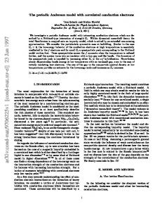
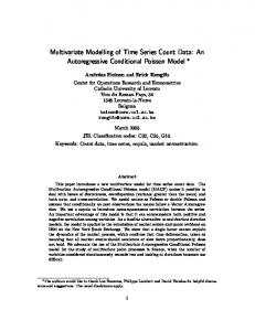
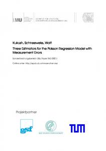
in Figures 1 and Figure 2, respectively. The posterior means and standard deviation (SD) of the residual, herd and sire variances affecting λ∗ were 0.76 (0.04), 0.36 (0.02) and 0.07 (0.01), respectively, with the most important source of variation being that due to residual effects, followed by herds and then by sires. In Figure 1, the posterior distributions of the residual and herd variances were nearly symmetric, while the posterior distribution of the sire variance was slightly asymmetric with a longer tail to the right. The posterior means (SD) of the residual, herd and sire variances affecting p∗ were 0.4 (0.11), 0.45 (0.13) and 0.27 (0.11), respectively, with the largest source of variation being herd effects, followed by residuals and then sires. As shown in Figure 2, the posterior distributions of the residual, herd and sire variances affecting p∗ were all skewed, with long tails to the right. These results suggest that it is more difficult to infer components of variance precisely for p∗ than for λ∗ . [Figure 1 about here.] [Figure 2 about here.] The posterior distribution of the covariance (correlation) between sire effects on λ∗ and p∗ is shown in Figure 1, with the mean (SD) of the sire covariance being 0.01 (0.02). The 90% credible interval is given by (−0.02; 0.05), suggesting that genetic effects affecting λ∗ and p∗ are uncorrelated. There was large uncertainty about the sire correlation (which is equal to the genetic correlation, under additive inheritance at the λ∗ and p∗ levels). The posterior distribution assigned high density to values of the correlation varying from −0.4 to 0.4. As shown in Figure 2, the distribution (over observations) of the posterior means of the perfect state probabilities p was skewed, and its mean (SD) was 0.07 (0.11); the 5% and 95% percentiles yielded the 90% interval (0.02; 0.22). This leads to the inference that, on average, about 7% of first-lactation cows would not get mastitis, either due to being totally resistant to the disease or for never being exposed to mastitis. The posterior predictive densities of the discrepancy statistic Dk displayed in Figure 3
14
Biometrics, 000 0000
(left panel) indicated that the predictive ability of the ZIP model is not entirely satisfactory. However, for number of cases of mastitis less or equal to 2, the agreement between observed and replicate data was close. The plot of posterior means of residuals displayed in Figure 3 (right panel) suggested that the model fitted the zero counts reasonably, but that it was less successful for fitting number of mastitis cases larger than 0 because the mean residual values were far from zero.
[Figure 3 about here.]
For comparative purposes, a Poisson model having the same exploratory structure for λ∗ was fitted to the data. In the Poisson model, the posterior means (SD) of the residual, herd and sire variances affecting λ∗ were 0.9 (0.03), 0.35 (0.02) and 0.05 (0.01), respectively. The residual variance was larger in the Poisson than in the ZIP model, suggesting that the overdispersion due to zeros was absorbed by the residual term in the Poisson model. The ZIP model captured more genetic variation, since the variation between sires was larger than in the Poisson model (posterior means were 0.07 and 0.05, respectively). Since the genetic correlation between λ∗ and p∗ was near zero, another ZIP model with σaλ,p = 0 was fitted. The mean (SD) of the posterior distribution of p in the uncorrelated and correlated ZIP models were 0.1 (0.11) and 0.07 (0.11), respectively. Estimates of the variance components affecting p∗ and λ∗ are summarized in Table 1. In general, estimates were similar, except for σa2p , where the mean was 37% larger (0.37 vs 0.27) in the uncorrelated ZIP model. Since the credible interval for the covariance between sire effects included zero, the principle of parsimony favors the uncorrelated ZIP model.
[Table 1 about here.]
A zero-inflated Poisson model with correlated parameters and application to animal breeding
15
4. Discussion Count data models have been developed for animal breeding applications, which pose either a Poisson mixed effects model (Foulley et al., 1987) or accommodate “extra-Poisson” residual variation explicitly (Tempelman and Gianola, 1996). However, part of this extra variation may be due to extra zeros relative to Poisson sampling. In this case, a ZIP model may provide a better fit to the data (Lambert, 1992). From an animal breeding perspective, quantities of main interest are the genetic values of candidates for selection and associated variance components. Here, the ZIP model was extended to accommodate genetic effects by introducing correlated random effects in the structure of the log-Poisson parameter (λ∗ ) and of the logit of the mixture probability (p∗ ). This structure is analogous to that of a multipletrait linear model described, for example, in Sorensen and Gianola (2002). Moreover, a correlation between these two genetic effects would account for pleiotropic genes affecting the Poisson and the mixture probability, as in models in which a correlation between direct and maternal effects is fitted (Willham, 1963). The hierarchical structures posed for λ∗ and p∗ would permit to discriminate between individuals being resistance to a certain disease and those that are mildly liable. In an application of this model to number of mastitis cases in first-lactation Norwegian Red cows, it seemed that a Poisson regression model absorbed overdispersion due to zeros in the residual term. If this is so, the Poisson mixed model would produce poorer estimates of the variance components. In the ZIP model, the components of variance affecting p∗ were inferred less precisely than those affecting λ∗ . Although the scale reduction factor value proposed by Gelman and Rubin (1992) was satisfied as a convergence criterion, trace plots (not shown here) suggested that, in the case of variance components affecting p∗ , additional iterations were needed for convergence. However, this can be computationally very intensive. Mixing might be improved by switching
16
Biometrics, 000 0000
sampling order of the unknowns at each iteration of the Gibbs-Metropolis algorithm as this would reduce the serial correlation between successively sampled quantities. The posterior correlation structure indicated a high correlation between the genetic variance affecting λ∗ and the genetic covariance (0.93); between the genetic variance affecting p∗ and genetic covariance (0.86), and between the genetic variances affecting λ∗ and p∗ (0.63). Another form of improving mixing would be via a blockwise Gibbs-Metropolis sampler, as proposed by Gelman et al. (2004). The fully conditional distributions of λ∗ and p∗ are not recognizable, so a MetropolisHastings scheme was needed to sample the appropriate unknowns. We found that a normal proposal distribution had a better performance than a random-walk proposal. It would be of interest to examine the performance of the Metropolis-Hastings scheme under different proposal distributions. Besag, York and Mollie (1991), working in a different problem, suggested that although a proper flat prior leads to a proper joint posterior distribution, it may produce a singularity invalidating the Gibbs sampler. This problem was not detected here, but a zero-mean normal prior with a large variance may be a better option.
Acknowledgements
Access to the data was given by the Norwegian Dairy Herd Recording System and the Norwegian Cattle Health Service in agreement number 004.2005. Research was funded by grants CAPES (BRAZIL) BEX 1758004, USDA 2003 − 35205 − 12833, NSF DEB-0089742 and NSF DMS 0443771. Support by the Wisconsin Agriculture Experiment Station and by the Babcock Institute for Dairy Research and Development is acknowledged.
References
Besag, J., York, J. and Mollie, A. (1991). Bayesian image restoration with two applications in spacial statistics. Annals of the Institute of Statistics and Mathematics 43, 1–59.
A zero-inflated Poisson model with correlated parameters and application to animal breeding
17
Carl´en, E., Schneider, M. del P. and Strandberg, E. (2005). Comparison between linear models and survival analysis for genetic evaluation of clinical mastitis in dairy cattle. Journal of Dairy Science 88, 797–803. Chang, Y. M., Gianola, D., Heringstad, B. and Klemetsdal, G. (2004). Effects of trait definition on genetic parameter estimates and sire evaluation for clinical mastitis threshold models. Animal Science 79, 355–363. Falconer, D. S. (1989). Introduction to Qunatitative Genetics, 3rd. edition. New York: Willey. Foulley, J. L., Gianola, D. and Im, S. (1987). Genetic evaluation of traits distributed as Poisson-binomial with reference to reproductive characters. Theoretical and Applied Genetics 73, 870–877. Gelman, A. and Rubin, D. B. (1992). Inference from iterative simulation using multiple sequences. Statistical Science 7, 457–511. Gelman, A., Carlin, J. B., Stern, H. S. and Rubin, D. B. (2004). Bayesian Data Analysis. London: Chapman and Hall. Gianola, D. and Foulley, J. L. (1983). Sire evaluation for ordered categorical data with a threshold model. Genetic, Selection, Evolution 15, 201–224. Heringstad, B., Rekaya, R., Gianola, D., Klemetsdal, G. and Weigel, K. A. (2001). Bayesian analysis of liability of clinical mastitis in Norwegian cattle with a threshold model: effects of data sampling method and model specification. Journal of Dairy Science 84, 2337– 2346. Heringstad, B., Chang, Y. M., Gianola, D. and Klemetsdal, G. (2003). Genetic analysis of longitudinal trajectory of clinical mastitis in first-lactation Norwegian cattle. Journal of Dairy Science 86, 2676–2683. Heringstad, B., Chang, Y. M., Gianola, D. and Klemetsdal, G. (2004). Multivariate threshold model analysis of clinical mastitis in multiparous Norwegian dairy cattle. Journal of
18
Biometrics, 000 0000
Dairy Science 87, 3038–3046. Lambert, D. (1992). Zero-inflated Poisson regression, with an application to defects in manufacturing. Technometrics 34, 1–14. Rodrigues-Motta, M., Gianola, D. , Heringstad, B., Rosa, G. J. M. and Chang. Y. M. (2007). A Zero-Inflated Poisson Model for Genetic Analysis of the Number of Mastitis Cases in Norwegian Red Cows. Journal of Dairy Science 90, 5306–5315. Sorensen, D. and Gianola, D. (2002). Likelihood, Bayesian, and MCMC Methods in Quantitative Genetics. Springer. Tempelman, R. J. and Gianola, D. (1996). A mixed effects model for overdispersed count data in animal breeding. Biometrics 52, 265–279. Willham, R. L. (1963). The covariance between relatives for characters composed of components contributed by related individuals. Biometrics 19, 18–27.
A zero-inflated Poisson model with correlated parameters and application to animal breeding
herd variance
0
0
2
5
10
Density
6 4
Density
8
15
10
residual variance
0.60
0.65
0.70
0.75
0.80
0.85
0.90
0.95
0.30
0.35
sire covariance
Density
0
0
5
10
15
40 30 20 10
Density
0.45
20
sire variance
0.40
0.04
0.06
0.08
0.10
0.12
0.14
−0.10
−0.05
0.00
0.05
0.10
0.15
Density
0.0 0.5 1.0 1.5 2.0 2.5
sire correlation
−0.6
−0.4
−0.2
0.0
0.2
0.4
0.6
Figure 1. Posterior distributions of the dispersion components affecting λ∗ and of sire covariances and correlations between λ∗ and p∗ .
19
20
Biometrics, 000 0000
herd variance
2.0 1.5
Density
1.0
2 0
0.0
0.5
1
Density
3
2.5
3.0
residual variance
0.2
0.4
0.6
0.8
1.0
0.2
0.4
0.8
1.0
mean of p
6
Density
0
0
2
1
4
2
Density
3
8
4
10
12
sire variance
0.6
0.2
0.4
0.6
0.8
1.0
0.0
0.2
0.4
0.6
0.8
1.0
Figure 2. Posterior distribution of the dispersion components affecting p∗ and distribution of the posterior means of the probability of the perfect state (p).
A zero-inflated Poisson model with correlated parameters and application to animal breeding
Distribution of the posterior means of the standardized residuals
−1
−0.10
0
1
residual means
0.00 −0.05
T(y|.)−T(y_rep|.)
2
0.05
3
0.10
Posterior distribution of the discrepancy statistic T(y|.)−T(y_rep|.)
0
1
2
3
number of mastitis cases
>=4
0
1
2
3
4
5
6
7
8
9
13
number of mastitis cases
Figure 3. Distribution of the discrepancy statistic, and of posterior means of the residuals under the correlated ZIP model.
21
22
Biometrics, 000 0000
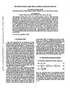
Table 1 Inference on residual (σε2λ , σε2p ), herd (σh2 λ ,σh2 p ) and sire (σa2λ ,σa2p ) variances affecting λ∗ and p∗ in ZIP models with or without genetic correlation between λ∗ and p∗ .
Posterior mean (standard error) Uncorrelated ZIP Correlated ZIP σε2λ σh2λ σa2λ σε2p σh2p σa2p
0.72 0.36 0.09 0.36 0.41 0.37
(0.04) (0.02) (0.01) (0.10) (0.13) (0.10)
0.76 0.36 0.07 0.40 0.45 0.27
(0.04) (0.02) (0.01) (0.11) (0.13) (0.11)