University of British Columbia Department of Statistics Technical Report #262 December 2010
“An invariant loss function for quantile approximation, estimation and summarizing data” by Reza Hosseini University of British Columbia
[email protected]
Department of Statistics, University of British Columbia
ABSTRACT This paper develops a loss function to assess the goodness of approximation or estimation of quantiles of a distribution (or data). We propose one that is invariant under monotonic transformations and we show by examples why this property is desirable in applications, in particular for making decisions that are invariant under (non-linear) change of scale of data. We show that the sample version of this loss function tends uniformly to the distributional version. This loss function can also be used to find optimal ways to summarize data (specially massive data), find equivariant ways to estimate quantiles and to define a measure of distance among random variables. We also show the usefulness of this loss function in interpreting results for quantiles. For example we show that even if the quantiles are not equivariant under increasing transformations and in fact the transformed quantile can be arbitrarily far from the quantile of the transformed random variable in terms of typical losses (such as absolute value), the distance is zero using this loss. It is also discussed how this loss function can be extended to multi-dimensions and statistics of data.
Keywords: Loss function; quantiles; invariant; large datasets; estimation; approximation
1
Introduction
This paper develops a “loss function” to assess the goodness of an approximation or an estimator of quantiles of a distribution (or a data vector). Suppose a quantile of a very large data vector, q is approximated by qˆ. Several classic losses can be considered. For example: absolute error L(q, qˆ) = |q − qˆ| or squared error L(q, qˆ) = (q − qˆ)2 which was proposed by Gauss. Quoting from [6]: “Gauss proposed the square of the error as a measure of loss or inaccuracy. Should someone object to this specification as arbitrary, he writes, he is in complete agreement. He defends his choice by an appeal to mathematical simplicity and convenience.” An obvious problem with this loss is its lack of invariance under (possibly non-linear) re-scaling of data. We propose a loss function that is invariant under strictly monotonic transformations. We also show that the sample version of this loss function tends uniformly to the distributional version. This loss function can be used also to find optimal ways to summarize a data vector and to define a measure of distance among random variables as discussed here. We define the loss of estimating/approximating q by qˆ to be the probability that the random variable falls in between the two values. A limited version of this concept only for data vectors can be found in computer science literature, where !approximations are used to approximate quantiles of large datasets (see for example [7]). However, this concept has not been introduced as a measure of loss and the definition is limited to data vectors rather than arbitrary distributions. Since we use quantiles in this paper, we give a definition (slightly different from the customary one) and a lemma that gives the elementary properties. The traditional definition of quantiles for a random variable X with distribution function F, lqX (p) = inf{x|F (x) ≥ p}, appears in classic works as [8]. We call this the “left quantile function”. In some books (e.g. [9]) the quantile is defined as rqX (p) = sup{x|F (x) ≤ p}, this is what we call the “right quantile function”. Also in robustness literature people talk about the upper and lower medians which are a very specific case of these definitions. [2] considers both definitions, explore their relation and shows that considering both has several advantages. He also proves the following lemma regarding the properties of the quantiles. Lemma 1.1 (Quantile Properties Lemma) Suppose X is a random variable on the probability space (Ω, Σ, P ) with distribution function F :
–2– a) F (lqF (p)) ≥ p. b) lqF (p) ≤ rqF (p). c) p1 < p2 ⇒ rqF (p1 ) ≤ lqF (p2 ). d) rqF (p) = sup{x|F (x) ≤ p}. e) P (lqF (p) < X < rqF (p)) = 0. i.e. F is flat in the interval (lqF (p), rqF (p)). f ) P (X < rqF (p)) ≤ p. g) If lqF (p) < rqF (p) then F (lqF (p)) = p and hence P (X ≥ rqF (p)) = 1 − p. h) lqF (1) > −∞, rqF (0) < ∞ and P (rqF (0) ≤ X ≤ lqF (1)) = 1. i) lqF (p) and rqF (p) are non-decreasing functions of p. j) If P (X = x) > 0 then lqF (F (x)) = x. k) x < lqF (p) ⇒ F (x) < p and x > rqF (p) ⇒ F (x) > p. For continuous variable [2] shows: Lemma 1.2 (Continuous distributions inverse) If F is continuous F (x) = p ⇔ x ∈ [lqX (p), rqX (p)]. Section 2 introduces the probability loss for data vectors by showing the motivation of the definition in terms of the “degree of separation” between data points in a sorted vector. Section 3 extends the definition to distribution functions and shows the elementary properties of this loss function under strictly increasing or decreasing transformations. This section also contains examples to show the usefulness of this loss specially in taking decisions that are invariant of the scale of data. Section 4 shows that the sample version of probability loss tends to the distribution version when the sample size goes to infinity which is an easy consequence of Glivenko-Cantelli Theorem. Section 5 shows the desirable properties of the probability loss when the underlying distribution function is continuous. For example in that case the probability loss satisfies the triangular inequality. Section 6 interprets many results about the quantiles and sample quantiles using the probability loss. For example even though the sample quantiles are not almost surely convergent to the distribution quantiles, they converge to the distribution quantile in terms of the probability loss. Also it is shown that even though quantiles of a distribution are not equivariant under strictly monotonic transformations, the probability loss of the transformed quantile and the quantile of the transformed random variable is zero. Section 7 studies how large the probability loss between two quantiles or a
–3– group of consequent quantiles can become when we change the underlying distribution function or data vector. This is useful when one wants to create quantile data summaries and so on using the probability loss as shown in [2] (Chapter 8). Section 8 introduces the “penalized” probability loss which is non-zero whenever the two values differ. It studies its properties and shows it satisfies the triangular inequality for appropriate penalties and also shows the choice of the penalty is not very influential in most cases. Section 9 discusses possible extensions of probability loss to multi-dimensions and statistics. Section 10 shows the applications of the probability loss in handling large data sets, summarizing them and inferring about their “exact quantiles” in the presence of missing values or contaminated data. It also shows how the probability loss can be used to approximate quantiles of large data sets specially when sorting the whole data set is not possible and the sorting can be done for smaller partitions. Section 11 shows how the probability loss can be used in estimating parameters (quantiles) of distributions in a framework similar to Wald decision theoretic approach with the desirable property that the estimators are equivariant under changes of scale of data (even non-linear). Finally Section 12 discusses other applications of the probability loss, for example in defining a measure of distance among random variables.
2
Probability loss for data vectors
Our purpose is to find good approximations to the median and other quantiles. We need a method to asses such approximations. We contend that such a method should not depend on the scale of the data. In other words it should be invariant under monotonic transformations. We define a function δ that measures a natural “degree of separation” between data points of a data vector x. For the sake of illustration, consider the example sort(x) = (1, 2, 3, 3, 4, 4, 4, 5, 6, 6, 7). Now suppose, we want to define the degree of separation of 3,4 and 7 in this example. Since 4 comes right after 3, we consider their degree of separation to be zero. There are 3 elements between 4 and 7 so it is appealing to measure their degree of separation as 3 but since the degree of separation should be relative, we also divide by n = 11, the length of the vector, and get: δ(4, 7) = 3/11. We can generalize this idea to get a definition for all pairs in R. With the same example, suppose we want to compute the degree of separation between 2.5 and 4.5 that are not members of the data vector. Then since there are 5 elements of the data vector between these two values, we define their degree of separation as 5/11. More formally, we give the following definition. Definition 2.1 Suppose x = (x1 , · · · , xn ), a data vector and z < z ! let ∆x (z, z ! ) = {i|z < xi < z ! , i = 1, · · · , n}. Then we define δx (z, z ! ) =
|∆x (z, z ! )| , n
–4– and δx (z, z) = 0, where |∆x (z, z ! )| is the cardinality of ∆x (z, z ! ). We call δx the “degree of separation” (DOS) or the “probability loss” associated with x. We then have the following lemma about the properties of δ. Lemma 2.1 The degree of separation δx has the following properties: a) δx ≥ 0. b) y < y ! < y !! ⇒ δx (y, y !! ) ≥ δx (y, y ! ). c) δφ(x) (φ(z), φ(z ! )) = δx (z, z ! ) if φ is a strictly monotonic transformation. d) y = sort(x) and yi < yj ⇒ δx (yi , yj ) ≤ (j − i − 1)/n. Proof Both a) and b) are straightforward. To show (c), suppose z < z ! and φ is strictly decreasing. (The strictly increasing case is similar.) Then φ(z ! ) < φ(z) and hence ∆φ(x) (φ(z), φ(z ! )) = {i|φ(z ! ) < φ(xi ) < φ(z)} = {i|z < xi < z ! } = ∆x (z, z ! ). Finally d) is true because |∆x (yi , yj )| = |{l|yi < xl < yj , l = 1, · · · , n}| ≤ j − i − 1. Remark. The definition and results above can be applied to random vectors S = (X1 , · · · , Xn ) as well. In that δS (z, z ! ) is random. To develop our theory, we need to study the asymptotic behavior of these statistics. We do so in later sections.
3
Probability loss for distributions
We define a degree of separation for distributions which corresponds to the notion of probability defined for data vectors to measure separation between data points. Definition 3.1 Suppose X has a distribution function F . Let δF (z ! , z) = δF (z, z ! ) = lim− F (u) − F (z ! ) = P (z ! < X < z), z > z ! , u→z
and δF (z, z) = 0, z ∈ R. We also denote this by δX whenever a random variable X with distribution F is specified. We call δX the “degree of separation” or the “probability loss” associated with X. The following lemma is a straightforward consequence of the definition. Lemma 3.1 Suppose x = (x1 , · · · , xn ) is a data vector with the empirical distribution Fn . Then δFn (z, z ! ) = δx (z, z ! ), z, z ! ∈ R.
–5– This lemma implies that to prove a result about the degree of separation of data vectors, it suffices to show the result for the degree of separation of random variables. Theorem 3.1 Let X, Y be random variables and FX , FY , their corresponding distribution functions. a) Assume Y = φ(X), for a strictly increasing or decreasing function φ : R → R. Then δFX (z, z ! ) = δFY (φ(z), φ(z ! )), z < z ! ∈ R. b) δFX (z, z ! ) ≤ δFX (z, z !! ), z ≤ z ! ≤ z !! . c) δFX (z1 , z3 ) ≤ δFX (z1 , z2 ) + δFX (z2 , z3 ) + P (X = z2 ). d) Suppose, p ∈ [0, 1]. Then δFX (lqFX (p), rqFX (p)) = 0. e) Suppose, p1 < p2 ∈ [0, 1]. Then δFX (lqFX (p1 ), rqFX (p2 )) ≤ p2 − p1 . Remark. We may restate Part (c), for data vectors: Suppose x has length n and z2 is of multiplicity m, (which can be zero). Then the inequality in (c) is equivalent to δx (z1 , z3 ) ≤ δx (z1 , z2 ) + δx (z2 , z3 ) + m/n. Proof a) Note that for a strictly increasing function φ, we have P (z < X < z ! ) = P (φ(z) < φ(X) < φ(z ! )). Now suppose φ is strictly decreasing. Then z < z ! ⇒ φ(z ! ) < φ(z). Let Y = φ(X). Then δX (z, z ! ) = P (z < X < z ! ) = P (φ(z ! ) < φ(X) < φ(z)) = δY (φ(z), φ(z ! )). b) This is trivial. c) Consider the case z1 < z2 < z3 . (The other cases are easier to show.) Then δFX (z1 , z3 ) = P (z1 < X < z3 ) = P (z1 < X < z2 ) + P (X = z2 ) + P (z2 < X < z3 ) = δFX (z1 , z2 ) + δFX (z2 , z3 ) + P (X = z2 ). d) This result is a straightforward consequence of Lemma 1.1 b) and c). e) This result follows from δFX (lq(p1 ), rq(p2 )) = P (lq(p1 ) < X < rq(p2 )) = P (X < rq(p2 )) − P (X ≤ lq(p1 )) ≤ p2 − p1 . The last inequality being a result of Lemma 1.1 a) and d). Remark: (e),(b) immediately imply δFX (lqFX (p1 ), lqFX (p2 )) ≤ p2 − p1 ,
–6– and δFX (rqFX (p1 ), lqFX (p2 )) ≤ p2 − p1 . Remark. We call Part c) of the above theorem the pseudo-triangle inequality. Here we give two examples about using the probability loss function and its interpretation. Example 1: We showed above that the triangle property does not hold for the probability loss function and that might lead to the criticism that this definition is not intuitively appealing. By an example, we now show why it makes sense that the triangle property should not hold for such a situation. Suppose a few mathematicians are standing in a line Euclid, Khawarzmi, Khayyam, Gauss, Von Neumann. If we were to ask Khwarzmi about his distance from Euclid, he would answer: “0, since I am right beside him.” If we ask Khwarazmi again about his distance to Khayyam, he will say that “my distance is 0 since I am right beside him.” However if we were to ask Euclid about his distance to Khayyam he would answer: “One unit (person) since Khwarzmi is in the middle.” We observe that this distance does not satisfy the triangle property as well. In this example the people sitting in the middle are the relevant factors. If we deal with a vector of sorted observations, then observations in the middle are the relevant factors. The following example shows the importance of invariance of loss (used to take a decision) under monotonic transformations. Example 2: A student is told that he will receive a scholarship if he ranks first in an exam in his class in either of the subjects mathematics and physics. The teacher of the courses differ and take a practice exam in each subject. They return the students back their marks out of 100. They also publish the lists of all the marks after removing the names, to give the students a feeling of how they did in the class. Table 1 shows the marks in mathematics and physics.
–7– Mathematics
Physics
Physics before re-scaling
80 65 63 61 54 54 53 50 49 48 47 47 46 44 30
90 89 86 85 83 82 79 79 76 75 72 72 69 68 55
81.0 79.2 74.0 72.2 68.9 67.2 62.4 62.4 57.8 56.2 51.8 51.8 47.6 46.2 30.2
Table 1: A class marks in mathematics and physics. The third column are the raw physics marks before the physics teacher scaled them. Sarina got 63 in math and 75 in physics. He decided to focus on just one subject that gives him a better chance in order to win the scholarship. He compared his mark in math with the best student in math: 63 against 80. So he needed |best mark − Sarina’s mark| = 80 − 63 = 17
more marks to be as good as the best student. Then he compared his physics mark to the best student in physics. He found he needs 90-75=15 marks to be as good as him. So he thought it’s better to focus on physics. But then he realized that different teachers use different exam and scoring methods. He had heard that the physics teacher scales the marks upward by the formula √ new mark = 100 × old mark. So the student calculated the untransformed values and put the result in the third column. Now he noticed that his new mark is 56.2 while the best mark is 91. The difference this time is 24.8 which is a larger difference than before. According to his “decision-making tool”, the absolute difference, he should focus on math since the absolute difference for math was only 17. But what if the mathematics teacher had used another transformation to re-scale the marks without him knowing it? This made him see a disadvantage to using the absolute value difference. Instead he realized, he can use the number of the students between himself and the best student as a measure of the difficulty of getting the best mark. He noticed his decision in this case will be independent of how the teachers re-scaled the marks. In the math case there is only one and for physics there are 8 students between him and the best student. Hence he decided that he should focus on math.
–8– This example shows in order to avoid contrary decisions when the scale changes, we need invariance of the loss under such transformations. This example was under the assumption that other students do not change their study habits or do not have access to the marks. If the other students had access to their marks or were ready to change their study focus, we need to take into account other possible actions of the other students and the problem will become game-theoretical in nature, a very interesting problem on its own right. The solution for that problem we conjecture to be the same.
4
Limit theory for probability loss function
Suppose a random variable X with a distribution function F is given and S = (X1 , · · · , Xn ) as an i.i.d sample from X and let Fn be the empirical distribution of the sample. We defined a distribution loss associated with F, δF a deterministic function and the loss associated to the sample δFn , a random variable. The following theorem shows the sample loss tends to the distribution loss almost surely. Theorem 4.1 Suppose X1 , X2 , · · · , is a sequence of i.i.d random variables with distribution function F . Then as n → ∞, δFn (z, z ! ) → δF (z, z ! ), a.s.,
uniformly in z, z ! ∈ R. In other words
sup |δFn (z, z ! ) − δF (z, z ! )| → 0, a.s..
z>z " ∈R
Proof If z = z ! , the result is trivial. Suppose z > z ! . We need to show that lim Fn (u) − Fn (z ! ) → lim− F (u) − F (z ! ),
u→z −
a.s. u→z
(1)
as n → ∞, uniformly in z > z ! ∈ R. Suppose ! > 0 is given. By Glivenko-Cantelli Theorem there exist N ∈ N such that for every n > N : ! |Fn (u) − F (u)| < , a.s., ∀u ∈ R. 2 Now for n > N , |( lim− Fn (u) − Fn (z ! )) − ( lim− F (u) − F (z ! ))| ≤ u→z
u→z
!
| lim− (Fn (u) − F (u))| + |Fn (z ) − F (z )| = lim− |Fn (u) − F (u)| + |Fn (z ! ) − F (z ! )|. u→z
!
u→z
But since |Fn (u) − F (u)| < 2" , limu→z− |Fn (u) − F (u)| ≤ 2" . Also |Fn (z ! ) − F (z ! )| < 2" . Hence |( lim− Fn (u) − Fn (z ! )) − ( lim− F (u) − F (z ! ))| < !. u→z
u→z
–9–
5
Probability loss for continuous distributions
This section studies the probability loss when the distribution function is continuous. The results are given in the following lemmas, which show some of its desirable properties in the continuous case. Lemma 5.1 (Probability loss for continuous distributions) Suppose X is a random variable with distribution function FX . Then δX (lqX (p1 ), rqX (p2 )) = p2 − p1 , p2 > p1 , ∀p1 , p2 ∈ [0, 1] if and only if FX is continuous. Proof If FX is continuous then for p1 < p2 and by Lemma 1.2, δ(lqX (p1 ), rqX (p2 )) = P (lqX (p1 ) < X < rqX (p2 )) = P (X < rqX (p2 )) − P (X ≤ lqX (p)) = F (rqX (p2 )) − F (lqX (p2 )) = p2 − p1 .
If F is not continuous then there exists an x0 such that a = PX (X = x0 ) > 0. Let p1 = P (X < x0 ) + a/3 and p2 = P (X < x0 ) + a/2. Clearly lqX (p1 ) = x0 and rqX (p2 ) = x0 . Hence δ(lqX (p1 ), rqX (p2 )) = 0 ,= p2 − p1 .
Lemma 5.2 Suppose δ(lqX (p1 ), rqX (p2 )) = δ(rqX (p1 ), lqX (p2 )) = a, p1 < p2 . Then also a = δ(lqX (p1 ), lqX (p2 )) = δ(rqX (p1 ), lqX (p2 )) = δ(rqX (p1 ), rqX (p2 )). Moreover, if X is continuous, all the above are equal to p2 − p1 . Proof The result follows immediately from the fact that all the three quantities are greater than or equal to δ(rqX (p1 ), lqX (p2 )) = a and smaller than or equal to δ(lqX (p1 ), rqX (p2 )) = a. The second part is straightforward using the previous lemma.
6
Interpreting results about quantiles using probability loss
This section shows the usefulness of probability loss for interpreting results about quantiles that do not appear intuitive under typical losses such as absolute or square error.
– 10 –
Closeness of left and right quantiles By definition left and right quantiles. The left and right quantile at a point p can disagree. In fact their absolute difference can become arbitrarily large. For example for k > 0 define P (X = 0) = P (X = k) = 1/2. Then lqX (1/2) = 0, rqX (1/2) = k and hence |lqX (1/2) − rqX (1/2)| = k, where k can be taken arbitrarily large. However, it is easy to see P (lqX (p) < X < rqX (p)) = 0 (Lemma 1.1, Part (e)) and we conclude δX (lqX (p), rqX (p)) = 0.
Convergence of sample quantiles We can consider the left and right quantiles of the empirical distribution function Fn of a sample X1 , · · · , Xn of independent random variables identically distributed with distribution function F . Then one would hope that lqFn → lqF (p) and rqFn (p) → rqF (p). This is actually true if lqF (p) = rqF (p). In fact one can show by an example that this is not true if lqF (p) = rqF (p). Moreover [3] showed if lqF (p) ,= rqF (p) then the sample quantiles diverge almost surely. More precisely he showed Theorem 6.1 (Quantile Convergence/Divergence Theorem) a) Suppose rqF (p) = lqF (p) then rqFn (p) → rqF (p), a.s., and lqFn (p) → lqF (p), a.s.. b) When lqF (p) < rqF (p) then both rqFn (p), lqFn (p) diverge almost surely. Proof See [3]. Unfortunately based on the above theorem the sample quantiles do not converge in general to the distribution version. In fact [3] shows that when lqF (p) < rqF (p) the liminf of the sample quantile is lqF (p) and the limsup is rqF (p). Moreover, [2] shows in the following theorem the nice property that in general the sample quantiles converge to distribution quantiles in the probability loss sense uniformly. In the following proof for a random variable X we define FXc (x) = P (X ≤ x) and FXo (x) = P (X < x). Theorem 6.2 Let X1 , X2 , · · · be an i.i.d. random sample drawn from an arbitrary distribution function F . Then (a)
sup δF (lqFn (p), lqF (p)) → 0., a.s.,
p∈(0,1)
– 11 – and (b)
!
p∈(0,1)
δF (lqFn (p), lqF (p)) → 0., a.s..
Proof We only need to prove (a) since (b) is a straightforward consequence of (a). Clearly lqFn (p) = Xi:n for p ∈ ((i − 1)/n, i/n], i = 1, 2, · · · , n. Also Fnc (Xi:n ) ≥ i/n and Fno (Xi:n ) ≤ (i−1)/n. Pick an N large enough in the Glivenko-Cantelli Theorem such that n > N ⇒ |Fn (x) − F (x)| < !, and |Fno (x) − F o (x)| < !, uniformly in x. Consider two cases: Case I: Xi:n < lqF (p). Then δF (lqFn (p), lqF (p)) = δF (Xi:n , lqF (p)) = F (lqF (p)) − F c (Xi:n ) ≤ F o (lqF (p)) − Fnc (Xi:n ) + ! ≤ p − i/n + ! ≤ !. o
Case II: Xi:n > lqF (p). Then δF (lqFn (p), lqF (p)) = δF (Xi:n , lqF (p)) = F (Xi:n ) − F c (lqF (p)) ≤ Fno (Xi:n ) + ! − p ≤ (i − 1)/n + ! − p ≤ !. o
Since this holds for i = 1, 2, · · · , n and (0, 1) = ∪i=1,2,··· ,n ( i−1 , i ], the supremum is n n also less than !.
Equivariance of quantiles It is claimed that the classic quantile function, i.e. the left quantile function, is equivariant under strictly increasing transformations ([5] and [1]). However, [4] showed that continuity is a necessary (and sufficient) condition for this to hold. A counterexample for the claim is given below. Counterexample: Suppose X is distributed uniformly on [0,1]. Then lqX (1/2) = 1/2. Now consider the following strictly increasing transformation " x −∞ < x < 1/2 φ(x) = . x + 5 x ≥ 1/2 Let T = φ(X) then the distribution of T is given by
– 12 – 0 t P (T ≤ t) = 1/2 t−5 1
t≤0 0 < t ≤ 1/2 1/2 < t ≤ 5 + 1/2 . 5 + 1/2 < t ≤ 5 + 1 t>5+1
It is clear form above that lqT (1/2) = 1/2 ,= φ(lqX (1/2)) = φ(1/2) = 5 + 1/2. In fact for any increasing but not left continuous function we can build an example as above. Moreover the example can be built in a way that the transformed quantile and the quantile of the transformation are arbitrarily far in terms of the absolute difference (replace 5 by k in above example). In the following theorem [4] showed that with continuity this problem is resolved. Theorem 6.3 (Quantile Equivariance Theorem) Suppose φ : R → R is non-decreasing. a) If φ is left continuous then lqφ(X) (p) = φ(lqX (p)). b) If φ is right continuous then rqφ(X) (p) = φ(rqX (p)).
Proof See [4]. It is unappealing that the equivariance property does not hold for arbitrary increasing transformations. However, [4] showed that using the probability loss a version of equivariance can be shown for such functions. Lemma 6.1 (Equivariance under non-decreasing transformations) Suppose X is a random variable with distribution function F and φ : R → R a non-decreasing transformation on R. Also let Y = φ(X). Then a) φ(lqX (p)) ∈ [lqY (p), rqY (p)] b) φ(rqX (p)) ∈ [lqY (p), rqY (p)]. Remark. We conclude δY (φ(lqX (p)), lqY (p)) = 0, and δY (φ(rqX (p)), rqY (p)) = 0.
– 13 –
7
The supremum of probability loss
This section investigates how large the probability loss can become under various scenarios. The results are given in the following lemmas. Lemma 7.1 Let F be the set of all univariate distribution functions. Then sup δF (lqF (p1 ), lqF (p2 )) = p2 − p1 , p2 > p1 , p1 , p2 ∈ (0, 1).
F ∈F
Proof This follows from the fact that δF (lqF (p1 ), lqF (p2 )) ≤ p2 − p1 in general, as shown in Lemma 3.1 and δF (lqF (p1 ), lqF (p2 )) = p2 − p1 for continuous variables. The same is true for data vectors as shown in the following lemma. Lemma 7.2 Suppose the supremum in the following is taken over all data vectors, then sup δx (lqx (p1 ), lqx (p2 )) = p2 − p1 , p2 > p1 , p1 , p2 ∈ (0, 1). x
Proof We know that δx (lqx (p1 ), lqx (p2 )) ≤ p2 − p1 . To show that the supremum attains the upper bound, let xn = (1, · · · , n). Then lqxn (p1 ) = [np1 ] or [np1 ] + 1. Also lqxn (p2 ) = [np2 ] or [np2 ] + 1. Then ∆, the number of elements of x between lqxn (p1 ) and lqxn (p2 ) satisfies: [np2 ] − [np1 ] − 1 ≤ ∆ ≤ [np2 ] − [np1 ] + 1 ⇒ np2 − 1 − np1 − 1 − 1 ≤ ∆ ≤ np2 − np1 + 1 ⇒ −3/n ≤ δxn (p1 , p2 ) − (p2 − p1 ) ≤ 1/n. This shows that δxn (p1 , p2 ) tends to p2 − p1 uniformly for all p1 < p2 ∈ [0, 1]. Lemma 7.3 Suppose p1 , p2 , · · · , pm ∈ [0, 1] and m = 2k. Then sup max{δx (lqx (p1 ), lqx (p2 )), δx (lqx (p3 ), lqx (p4 )), · · · , δx (lqx (pm−1 ), lqx (pm ))} x
= max{|p2 − p1 |, · · · , |pm − pm−1 |}.
– 14 – Proof The supremum is less than or equal to the left hand side by Lemma 1.1. Let xn = (1, 2, · · · , n). Without loss of generality suppose p1 < p2 , p3 < p4 , · · · , p2k−1 < p2k . By the properties of quantiles of data vectors: lqxn (pi ) = x[npi ] = [npi ] or lqxn (pi ) = x[npi ]+1 = [npi ] + 1. Also, lqxn (pi+1 ) = x[npi+1 ] = [npi+1 ] or lqxn (pi+1 ) = x[npi+1 ]+1 = [npi+1 ] + 1. Then, δxn (lqxn (pi ), lqxn (pi+1 )) ≥ n1 ([npi+1 ] − [npi ] − 1) ≥ n1 (npi+1 − npi − 2) = (pi+1 − pi ) − n2 . Hence δxn (lqxn (pi ), lqxn (pi+1 )) > |pi+1 − pi | −
2 , i = 1, · · · , m − 1. n
The inequality shows the supremum is greater than = max{|p2 − p1 | −
2 2 , · · · , |pm − pm−1 | − }, n n
for all n ∈ N. Now let n → +∞ to get the conclusion.
Lemma 7.4 Suppose p1 , p2 , · · · , pm ∈ [0, 1] and a1 , a1 , · · · , a2m ∈ [0, 1]. Then ! a2 ! a4 δx (lqx (p2 ), lqx (p))dp+ sup[ δx (lqx (p1 ), lqx (p))dp + x
=
!
a3
a1
··· + a2 a1
!
|p − p1 |dp +
a2 m
δx (lqx (pm ), lqx (p))dp] a2m−1
!
a4 a3
|p − p2 |dp + · · · +
!
a2 m a2m−1
|p − pm |dp.
Proof The proof is similar to the previous lemmas and we skip the details.
8
penalized probability loss
This section introduces a family of loss functions that are very similar to the probability loss function but might be more useful in some contexts, particularly when the distribution function is not continuous. A defect of the probability loss function is: it can be equal to zero even if a ,= b, a, b ∈ R. Also we noted that even though it resembles a metric it is not one. For example the triangular inequality does not hold. We introduce the “c-probability loss” to solve these problems.
– 15 – Definition 8.1 Suppose X is a random variable, δX its associated probability loss function and c ≥ 0. Then let c δX (a, b) = δX (a, b) + c(1 − 1{0} (a − b)),
where 1{0} is the indicator function at zero. Note that the c-probability loss is the sum of two losses. The first, δX (a, b), is the probability of being between the two values (a and b), the second, c(1 − 1{0} (a − b)), is the penalty for a and b not being equal. One question is what value of c should be chosen as the “penalty” of not being equal to the true value. It turns out that the value of c is not very important for many purposes as shown in the following lemma. Lemma 8.1 (Properties of the c-probability loss functions) c a) δX (a, b) = c ⇔ a ,= b and δX (a, b) = 0. c c b) δX (a, b) = 0 or δX (a, b) ≥ c. c c) δX is invariant under strictly monotonic transformations. d) Let d = sup P (X = x0 ). Then if c ≥ d, δ c satisfies the triangle inequality. x0 ∈R
c e) δX (lqX (p), rqX (p)) ≤ c. (It is either zero or c.) c d f ) Suppose δX is given for any c > 0. Then we can obtain any other δX for d ≥ 0.
Proof a) and b) are trivial. c) Both δX and c(1 − 1{0} (a − b)) are invariant under monotonic transformations. d) We use the pseudo-triangle inequality for the probability loss function. Take c c c z1 , z2 , z3 ∈ R. We need to show δX (z1 , z3 ) ≤ δX (z1 , z2 ) + δX (z2 , z3 ) . If z1 = z3 , the result is trivial. Otherwise c(1 − 1{0} (z1 − z3 )) = c and c δX (z1 , z3 ) = δX (z1 , z3 ) + c ≤ δX (z1 , z2 ) + δX (z2 , z3 ) + P (X = z2 ) + c
≤ δX (z1 , z2 ) + δX (z2 , z3 ) + c(1 − 1{0} (z1 − z2 )) + c(1 − 1{0} (z2 − z3 )) = c c δX (z1 , z2 ) + δX (z2 , z3 ).
e) Trivial by properties of lq, rq and δX as shown in Lemma 1.1. c c d f) Suppose δX is given. If δX (a, b) = 0 then a = b and hence δX (a, b) = 0. If a ,= b c c (a, b) − c and then δX (a, b) = δX (a, b) + c. From this we can obtain δX (a, b) = δX c d hence δX (a, b) = δX (a, b) − c + d. i.i.d
c δX (X1 , X2 ) (or δX (X1 , X2 )), if X1 , X2 ∼ X can be considered as a measure of disparity of the common distribution. The following lemma shows that the expectation of this quantity is constant for all continuous random variables. It is also easy to show in the non-continuous case the expectation is smaller than the one given below.
– 16 – Lemma 8.2 Suppose X is a continuous random variable, then E(δX (X1 , X2 )) = 2/3, i.i.d
where X1 , X2 ∼ X. Also c E(δX (X1 , X2 )) = 2/3 + c.
Proof We know that FX (X1 ) and FX (X2 ) are both uniformly distributed on (0,1) and independent. Hence !
1 0
2
!
! 1
0
1 0
E(δX (X1 , X2 )) = E(|F (X1 ) − F (X2 )|) = ! 1! 1 |p1 − p2 |dp1 dp2 = 2 (p1 − p2 )dp1 dp2 = 0
p2
(1 − 2p2 + p22 )dp2 = 2/3.
c E(δX (X1 , X2 )) = 2/3 + c is obtained by noting that P (X1 = X2 ) = 0 for continuous random variables. It is interesting to note that δF (X1 , X2 ) in this case is a special case of the coverage probabilities discussed by [10].
9
Extensions to statistics and multi-dimensional data
This section shows how probability loss function can be extended to more than one dimension and also to measure the distance between statistics. However, we do not study this case in details and the applications are left to future research. Suppose X1 , · · · , Xn is a random sample and consider two statistics T1 (X1 , · · · , Xn ) and T2 (X1 , · · · , Xn ). For example these statistics might be estimators of lqX (p) e.g. Xi:n (ith order statistics) for some i. Then we can consider the random loss δX (T1 (X1 , · · · , Xn ), T2 (X1 , · · · , Xn )). In order to find optimal estimators we need a deterministic measure and one can settle for the expected probability loss (EPL) E(δX (T1 (X1 , · · · , Xn ), T2 (X1 , · · · , Xn ))). In the following definition we offer a new idea to measure this loss.
– 17 – Definition 9.1 Suppose X1 , X2 , · · · a random sample drawn from distribution function FX and consider another draw XF which is independent of the random sample (can think of this as a “future value”). Then for two statistics T1 (X1 , X2 , · · · ), T1 (X1 , X2 , · · · ), define the future value probability loss function (FPL) as follows γX (T1 , T2 ) = P (T1 < XF < T2 ) + P (T2 < XF < T1 ). Remark. Note that for constant numbers a, b we have γX (a, b) = δX (a, b). It can easily be shown that if S, T are equivariant under strictly monotonic transformations of the random sample then so is the FPL. Lemma 9.1 Suppose X1 , X2 , · · · a random sample from FX and XF is another draw independent from the random sample and consider a strictly monotonic transformation of the reals φ : R → R. If T1 (X1 , X2 , · · · ), T2 (X1 , X2 , · · · ), are two equivariant statistics under φ i.e. φ(Tj (X1 , X2 , · · · )) = Tj (φ(X1 ), φ(X2 ), · · · ), j = 1, 2 then we have γφ(X) (T1 (φ(X1 ), · · · ), T2 (φ(X2 ), · · · )) = γX (T1 (X1 , · · · ), T2 (X1 , · · · )) Remark. Order statistics clearly satisfy the above property. Remark. As a less trivial example consider a sample of size n = n1 + n2 : X1 , · · · , Xn1 , Y1 , · · · , Yn2 and consider min(Xi:n1 , Yj:n2 ). As yet a more interesting example let Z1 = Xi1 :n1 , · · · , Zk = Xik :n1 , Zk+1 = Yj1 :n2 , · · · , Zk+l = Yjl :n2 and consider Zs:(k+l) . This example has important applications in dealing with massive data sets. Suppose n1 , n2 are very large and hence loading the two sample in the same time on the computer memory is not possible, then one can 1-load them individually, 2-save a subset of their order statistics of size k and l and 3-use these summaries to infer about order statistics of the full sample or quantiles of the underlying distributions. It is also interesting to find optimal ways to choose these subsets.
– 18 – As an application, we can estimate a quantile lqX (p) using a statistics T . Then the loss can be assessed by either EPL or FPL. In fact in Section 11, we use these losses to find optimal estimators. Extensions to multi-dimensional data is possible in several ways. We introduce two ways here. In the first one, we extend the point loss definition defined on pairs of points in R to multi-dimensional pairs of points in Rk . Suppose X = (X 1 , · · · , X k ) a random vector in Rk and a = (a1 , · · · , ak ), b = (b1 , · · · , bk ) ∈ Rk then we can define δX (a, b) = P (X i ∈ (ci , di ), i = 1, · · · , k),
where ci = min(ai , bi ) and di = max(ai , bi ). Obviously this matches with the definition previously given for k = 1. We can again show the invariance property of this loss under componentwise strictly monotonic transformations φ = (φ1 , · · · , φk ) : Rk → Rk ,
meaning each φi : R → R is strictly monotonic. Another way to extend the definition is to consider a class “parallel” hyper surfaces in Rk (every two hyper surface in the class are identical or disjoint) and for two hyper surfaces S1 and S2 define the loss as the probability the random variable falls in between the two hyper surfaces. Such a class will be transformed to another class of parallel hyper surfaces using a componentwise strictly monotonic transformations. We leave the study of the properties of these extensions and applications to multi-variate data to future research.
10
Applications in approximating quantiles in large or imperfect datasets
First we prove two lemmas. These lemmas show what happens to the quantiles if we throw away a small portion of the data vector or add some more data to it. The first lemma is for a situation that we have thrown away or ignored a small part of the data. The second lemma is for a situation that a small part of the data are contaminated or includes outliers. In both cases, we show how the quantiles computed in the “imperfect” vectors correspond to the quantiles of the original vector. In both case x stands for the imperfect vector and w is the complete/clean data. Lemma 10.1 (Missing data quantile approximation lemma) Suppose x = (x1 , · · · , xn ), sort(x) = (y1 , · · · , yn ) and y ! = lqx (p), p ∈ [0, 1]. Consider a vector x# of length n# and let w = stack(x, x# ). Then y ! = lqw (p! ), where p! ∈ n! ! [p − !, p + !] and ! = n+n ! . In other words δw (y, y ) ≤ !. Similarly if y ! = rqx (p) and p ∈ [0, 1], y ! = rqw (p! ), where p! ∈ [p − !, p + !] n! ! and ! = n+n ! . δw (y, y ) ≤ !.
– 19 – Remark. Note that no error guarantee can be given using typical loss functions such as absolute value. Proof We prove the result for lqx only and a similar argument works for rqx . Let z = sort(w) then lqz = lqw . For p = 1 the result is easy to see. Otherwise, i ≤ p < i+1 for some i = 0, · · · , n − 1. But then y ! = lqx (p) = yi . In the new n n vector z since we have added n# elements y ! = zj for some j, i ≤ j < i + n# . Hence j y ! = lqz ( n+n ! ). From np − 1 < i ≤ np, we conclude np − 1 i j i + n# np + n# < ≤ < ≤ . n + n# n + n# n + n# n + n# n + n# Hence,
!
n# (1 − p) − 1 j n# (1 − p) < −p< ⇒ n + n# n + n# n + n# j n# (1 − p) − 1 n# (1 − p) | − p| < max{| |, | |}. n + n# n + n# n + n# !
(1−p) n n But | nn+n ! | ≤ n+n! and | conclude that that
! (1−p)−1
n+n!
|
!
n −1 1 | ≤ max{ n+n ! , n+n! } since p ranges in [0, 1]. We
j n# − p| < . n + n# n + n#
Lemma 10.2 (Contaminated data quantile approximation lemma) Suppose x = (x1 , · · · , xn ), sort(x) = (y1 , · · · , yn ) and y ! = lqx (p), p ∈ [0, 1]. Consider the vector w = (x1 , x2 , · · · , xn−n! ) then y ! = lqw (p! ), where p! ∈ [p − !, p + !] and n! ! ! = n−n ! . δw (y, y ) ≤ !. Similarly if y ! = rqx (p) and p ∈ [0, 1], y ! = rqw (p! ), where p! ∈ [p − !, p + !] n! ! and ! = n−n ! . δw (y, y ) ≤ !. Proof We only show the case for lqx and a similar argument works for rqx . Let z = sort(w). Then lqz = lqw . If p = 1 the result is easy to see. Otherwise, i ≤ p < i+1 for some i = 0, · · · , n − 1. But then y ! = lqx (p) = yi . In the new n n vector z since we have removed n# elements y ! = zj for some j, i − n# ≤ j ≤ i. j # Hence y ! = lqz ( n−n ! ). From np − 1 < i ≤ np, we conclude np − 1 − n < j ≤ np ⇒ np − n# ≤ j ≤ np. Hence −n# + n# p j n# p ≤ − p ≤ ⇒ n − n# n − n# n − n# |
n# j − p| ≤ . n − n# n − n#
– 20 – [2] introduced an algorithm to approximate quantiles of very large datasets. The idea of the algorithm is to read partitions of a very large data vectors sequentially and save a summary of the partitions and then refer about the quantiles of the original vector using the summaries. The algorithm allows for non-equal partition sizes. The accuracy of the approximation can be given deterministically using the probability loss function as stated in the following theorem. 'm Theorem 10.1 Suppose x is of length n = i=1 li , m ≥ 2 and li = ci d. Let 'm C = i=1 ci . Apply the “coarsening algorithm” ([2]) to x and find µ to approximate rqx (p) (or lqx (p)). Then µ is a (left and right) quantile in the interval [p − !, p + !], m+1 where ! = C−m . In other words δx (µ, rqx (p)) ≤ ! and δx (µ, lqx (p)) ≤ !. When m+1 1 3 li = cd, i = 1, · · · , m, ! = m−1 ≤ c−1 . c−1
Remark. Note that again no error guarantee can be given using typical loss functions such as absolute value.
11
Estimation
This section shows how the probability loss idea can be used to estimate parameters of a distributions, in particular quantiles. Here we discuss estimating a quantile of a random variable only. However, the method can be used in estimating parameters of any family of random variables that are specified by their quantiles at specific points. For example the normal family, N (µ, σ 2 ), can be specified by lq(0) = µ, lq(1) = µ + σ 2 and we call such families quantile-specified families. It can be seen that most of typical families of distributions are characterized by their values on specific quantiles. The idea is much the same as Wald’s decision theoretic approach ([6]) except for the loss is defined differently using expected probability loss δ. In fact we can avoid using expectation by using future probability loss. [2] showed that this estimation method is equivariant under changes of scale of data (even non-linear), a property that does not hold for typical loss functions such as the square error. Here we only focus on estimating a specific quantile and for simplicity suppose the distribution function is continuous and strictly increasing (Hence lq(p) = rq(p) = q(p)). However, by some modifications the results can re-stated for the general case. Suppose a random sample X1 , · · · , Xn and class of estimators are given D to estimate a quantile q(p). Then we propose to minimize either of the losses: a. Expected probability loss: argminD∈D EP L(D, q(p)) = argminD∈D E(δF (D, q(p))).
– 21 – b. Future probability loss: argminD∈D F P L(D, q(p)) = argminD∈D γF (D, q(p)). [2] shows such estimators are equivariant (if D is closed under strictly monotonic transformations). It is natural to consider D to include the order statistics X1:n , · · · , Xn:n (from the smallest to largest) functions F1:n , · · · , Fn:n . Also define ) j distribution 'n (nwith (n−j) Gi:n (y) = Fi:n (q(y)) = j=i j y (1 − y) . Then for D = Xi:n : a. We have
E(δF (Xi:n , q(p))) = E|F (Xi:n ) − p| = =
!
1 0
|p − y|dGi:n =
!
!
∞ −∞
p 0
(p − y)dGi:n +
!
|p − F (x)|dFi:n
1 p
(y − p)dGi:n .
b. We have
=
!
γF (D, q(p)) = P (Xi:n < XF < q(p)) + P (q(p) < XF < Xi:n ) ! +∞ ! +∞ = P (x < XF < q(p))dFi:n + P (q(p) < XF < x)dFi:n −∞
q(p) −∞
(p − F (x))dFi:n +
!
−∞
+∞
q(p)
(F (x) − p)dFi:n =
!
p
0
(p − y)dGi:n +
!
1
p
(y − p)dGi:n
Note that the estimator does not depend on the distribution as Gi:n is the same for all continuous random variables and hence invariant under (possibly nonlinear) changes of scale of data. It can also be shown that in the general (possibly non-continuous) these losses are equal to or smaller than the above. Interestingly in this case the two methods give rise to the same answer. Note that the solution does need to be unique. For example if p = 1/2 and n = 2 as it should be the case both X1:2 and X2:2 are equally eligible. These equations can be solved numerically (or by simulations) for any given n and i, however a theoretical solution is desirable and is left for future research.
12
Other applications
We saw before that the probability loss function is invariant under re-scaling of data. This is of great importance since the results obtained by using this loss function do not depend on the scale of the data as they should not in most applications. We also showed how this loss can be used to assess quantile approximations in large or imperfect datasets. We found bounds on the error of quantile approximations in
0.0
0.2
0.4
F(x)
0.6
0.8
1.0
– 22 –
−3
−2
−1
0
1
2
3
x
Figure 1: Comparing the standard normal distribution (solid) with optimal Cauchy picked by quantile distance (dashed) and the optimal Cauchy picked by tail quantile distance minimization (dotted). such datasets in terms of the probability loss. It can be easily seen that no such bound can be found using other classic measures of loss such as the absolute difference or the square of the difference (Since they are not invariant under monotonic transformations). [2] uses this loss function in many other applications and we point out some of them here. • Suppose a large data vector of length n is given. We want to find m