Jan 5, 2017 - [7] Aydin Buluç, Henning Meyerhenke, Ilya Safro, Peter Sanders, and Christian Schulz. ... [25] Alex Pothen, Horst D. Simon, and Kan-Pu Liou.
Abilities and Limitations of Spectral Graph Bisection Martin R. Schuster1 and Maciej Li´skiewicz1
arXiv:1701.01337v1 [cs.DS] 5 Jan 2017
1
Institute of Theoretical Computer Science, University of L¨ ubeck, Germany
Spectral based heuristics belong to well-known commonly used methods for finding a minimum-size bisection in a graph. The heuristics are usually easy to implement and they work well for several practice-relevant classes of graphs. However, only a few research efforts are focused on providing rigorous analysis of such heuristics and often they lack of proven optimality or approximation quality. This paper focuses on the spectral heuristic proposed by Boppana almost three decades ago, which still belongs to one of the most important bisection methods. It is well known that Boppana’s algorithm finds and certifies an optimal bisection with high probability in the random planted bisection model – the standard model which captures many real-world instances. In this model the vertex set is partitioned randomly into two equal sized sets, and then each edge inside the same part of the partition is chosen with probability p and each edge crossing the partition is chosen with probability q, with p ≥ q. In our paper we investigate the problem if Boppana’s algorithm works well in the semirandom model introduced by Feige and Kilian. The model generates initially an instance by random selection within the planted bisection model, followed by adversarial decisions. Feige and Kilian posed the question if Boppana’s algorithm works well in the semirandom model and it has remained open so far. In our paper we answer the question affirmatively. We show also that the algorithm achieves similar performance on graph models which generalize the semirandom model. On the other hand we prove some √ limitations of √ Boppana’s algorithm: we show that if the density difference p−q ≤ o( p · ln n/ n) then the algorithm fails with high probability in the√planted bisection model. This √ bound is sharp, since under assumption p − q ≥ Ω( p · ln n/ n) Boppana’s algorithm works well in the model.
1 Introduction The minimum graph bisection problem is one of the classical NP-hard problems [19]: for an undirected graph G the aim is to partition the set of vertices V = {1, . . . , n} (n even) into two equal sized sets, such that the number of cut edges, i.e. edges with endpoints in different bisection sides, is minimized. The bisection width of a graph G, denoted by bw(G), is then the minimum number of cut edges in a bisection of G. Due to practical and theoretical importance, the problem has been the subject of a considerable amount of research from different perspectives: approximation complexity [26, 2, 17, 16], parameterized algorithms [24, 31, 13] and average-case complexity [6]. Since the bisection problem is very hard in general – no polynomial-time algorithm is known even for approximating the minimum bisection to within a constant factor – an extensive research has been carried out to explore implementable heuristics that might be applied for wide, practice-relevant classes of graphs. Existing methods range from simple greedy techniques over flow algorithms [6] to spectral graph theory [25] and semidefinite programming [1]. A current survey of various bisection heuristics and common software packages is provided in [7]. In this paper we consider polynomial-time heuristics that for an input graph either output the minimum-size bisection or “fail”. In addition, for the output bisection, they give a proof that the bisection is optimal. The heuristics should work well for all (or almost all, depending on the model) realistic graphs, i.e. provide for them a certified optimum bisection, while for irregular, worst case instances the output can be “fail”, what is justifiable. In this paper we investigate two well-studied graph models which, as commonly believed, capture many realworld instances: The planted random model of Bui, Chaudhuri, Leighton and Sipser [6] and the semirandom model of Blum and Spencer [3] and Feige and Kilian [15]. Moreover, we consider the regular graph model introduced of Bui et al. [6] and a new extension of the semirandom model. For a (semi)random model of graphs we say that some property is satisfied with high probability (w.h.p.) if the probability that the property holds tends to 1 as the number of vertices n → ∞. In the planted bisection model, denoted as Gn (p, q) with parameters 1 > p = p(n) ≥ q(n) = q > 0, the vertex set V = {1, . . . , n} is partitioned randomly into two equal sized sets V1 and V2 , called the planted bisection. Then for every pair of vertices do independently: if both vertices belong to the same part of the bisection (either both belong to V1 or both belong to V2 ) then include an edge between them with probability p; If the two vertices belong to different parts, then connect the vertices by an edge with probability q. In the semirandom model for graph bisection [15], initially a graph G is chosen at random according to model Gn (p, q). Then a monotone adversary is allowed to modify G by applying an arbitrary sequence of the following monotone transformations: (1) The adversary may remove from the graph any edge crossing a minimum bisection; (2) The adversary may add to the graph any edge not crossing the bisection. Finally, in the regular random model, denoted as Gn (r, b), with r = r(n) < n and b = b(n) ≤ (n/2)2 , the probability distribution is uniform on the set of all graphs on V that are r-regular and have bisection width b. The main focus of our work is the bisection algorithm proposed by Boppana [5]. Though introduced almost three decades ago, the algorithm belongs still to the most important heuristics in this area. However, several basic questions concerning the algorithm’s performance remain open. Using a spectral approach, Boppana constructs an implementable algorithm
1
which, assuming the density difference p √ p − q ≥ Ω( p ln n/ n)
(1)
bisects Gn (p, q) optimally w.h.p. Remarkably, for a long time this was the largest subclass of graphs Gn (p, q) for which a minimum bisection could be found. The algorithm works well also on the regular graph model Gn (r, b), assuming that r ≥ 6 and
b ≤ o(n1−1/⌊(r+1)/2⌋ ).
(2)
In this paper we investigate the problem if, under assumption (1), Boppana’s algorithm works well for the semirandom model. This question was posed by Feige and Kilian in [15] and remained open so far. Most recently, Makarychev, Makarychev, and Vijayaraghavan [23, Sec. 1.2] have claimed (without a proof) that spectral algorithms do not work for this model. In our paper we answer Feige and Kilian’s question affirmatively which disproves the claim of Makarychev et al. We show also that Boppana’s algorithm achieves similar performance on graph models which generalize the semirandom model of [15]. On the other hand we show some limitations of the algorithm. One of the main results in this √ √ direction is that the density difference (1) is tight: we prove that if p−q ≤ o( p · ln n/ n) then the algorithm fails on Gn (p, q) w.h.p. Up to our best knowledge this is the first impossibility result for the random planted bisection model. Our Results. The motivation of our research was to systematically explore graph properties which guarantee that Boppana’s algorithm outputs a (certified) optimum bisection. Due to [5] we know that random graphs from Gn (p, q) and Gn (r, b) satisfy such properties w.h.p. under assumptions (1) and (2) on p, q, r, and b as discussed above. But, as we will see later, the algorithm works well also for instances which deviate significantly from such random graphs. Our first technical contribution is a modification of the algorithm to cope with graphs of more than one optimum bisection, like e.g. hypercubes. The algorithm proposed by Boppana does not manage to handle such cases. Our modification is useful to work on wider classes of graphs. In this paper we introduce a natural generalization of the semirandom model of Feige and Kilian [15]. Instead of Gn (p, q), we start with an arbitrary initial graph model Gn , and then apply a sequence of the transformations by a monotone adversary as in [15]. We denote such a model by A(Gn ). One of our main positive results is that if Boppana’s algorithm outputs the minimum-size bisection for graphs in Gn w.h.p., then the algorithm finds a minimum bisection w.h.p. for the adversarial graph model A(Gn ), too. As a corollary, we get that under assumption (1), Boppana’s algorithm works well in the semirandom model, denoted here as A(Gn (p, q)), and, assuming (2), in A(Gn (r, b)) – the semirandom regular model. To analyze limitations of the spectral approach we provide structural properties of the space of feasible solutions searched by the algorithm. This allows us to prove that if an optimal bisection contains some forbidden subgraphs, then Boppana’s algorithm fails. Using these tools, we were able to show that if the density difference p − q is asymptotically smaller than √ √ p · ln n/ n then Boppana’s algorithm fails on Gn (p, q) w.h.p. Since the behavior of the algorithm on the (common) semirandom model A(Gn (p, q)) remained unknown so far, Feige and Kilian proposed in [15] a new semidifinite programminig based approach which works for semirandom graphs, assuming (1). For a given graph G they define a minimization semidefinite program (SDP) with the objective function hp (G) and
2
prove that hd (G), which is the objective function of the dual maximization SDP, w.h.p. reaches bw(G) on graphs in Gn (p, q). On the other hand they show that hp (G) ≤ bw(G) and that hp preserves minimal bisection regardless of monotone adversary transformations. The proposed algorithm solves in polynomial time the primal SDP and reconstructs a certified minimum-size bisection of G from a feasible solution attaining optimum hp (G). A proof that the algorithm works well on A(Gn (p, q)) follows from inequalities hd (G) ≤ hp (G) ≤ bw(G) and the property that hd (G) = bw(G) w.h.p. The relationship between the performance of the SDP based algorithm and Boppana’s approach was left in [15] as an open problem. Feige and Kilian conjecture that for every G, the function hp (G) and the lower bound computed in Boppana’s algorithm give the same value. In our paper we answer this question affirmatively. To compare the algorithms, we provide a primal SDP formulation for Boppana’s approach and prove that it is equivalent to the dual SDP of Feige and Kilian. Next we give a dual program to the primal formulation of Boppana’s algorithm and prove that the optima of the primal and dual programs are equal to each other. Note that unlike linear programming, for semidefinite programs there may be a duality gap. An important advantage of the spectral method by Boppana over the SDP based approach by Feige and Kilian is that the spectral method is practically implementable reducing the bisection problem for graphs with n vertices to computing minima of a convex function of n variables while Feige and Kilian’s algorithms needs to solve a semidefinite program over n2 variables. Related Work. Spectral partitioning goes back to Fiedler [18], who first proposed to use eigenvectors to derive partitions. Spielman and Teng e.g. showed, that spectral partitioning works well on planar graphs [27, 28], although there are also graphs on which purely spectral algorithms perform poorly, as shown by Guattery and Miller [21]. Although spectral partitioning works well, providing a guarantee for the solution to be optimal is hard. Some progress could be made explicitly for the planted bisection random graph model: Coja-Oghlan developed a new spectral algorithm [9] which enables for a wider range of parameters in the planted bisection model than the generic algorithm of Boppana. Latest research by Coja-Oghlan et al. provides better understanding of the planted bisection model [11] and average case behaviour of a minimum bisection. Still the beforementioned algorithms stay the best for certifying partitions. Also other algorithms have been proven to work on the planted bisection model. Condon and Karp [12] developed a linear time algorithm for the more general l-partitioning problem. Their algorithm finds the optimal partition with probability 1 − exp(−nΘ(ε) ) in the planted bisection model with parameters satisfying p − q = Ω(1/n1/2−ε ). Carson and Impaglizzo [8] show that a hill-climbing algorithm is able to find the planted bisection w.h.p. for parameters p − q = Ω((ln3 n)/n1/4 ). The paper is organized as follows. The next section contains an overview over Boppana’s algorithm. In Section 3 we propose a modification of the algorithm to deal with non-unique optimum bisections. In Section 4 we define the adversarial graph model and show, that Boppana’s algorithm works well on this class. Next we develop a new analysis of the algorithm and use it to show some limitations of the method. Finally, in Section 6 we compare the algorithm to the SDP approach of Feige and Kilian. We conclude the paper with a discussion. The proofs of most of the propositions presented in Sections 2 through 6 are moved to the appendix (Section 8).
3
2 Boppana’s Graph Bisection Algorithm In this section we fix definitions and notations used in our paper and we recall Boppana’s algorithm and known facts on its performance. We need the details of the algorithm to describe its extension in the next section. For a given graph G = (V, E), with V = {1, . . . , n}, Boppana defines a function f for all real vectors x, d ∈ Rn as P P 1−x x (3) f (G, d, x) = {i,j}∈E 2i j + i∈V di (x2i − 1). P Call by S ⊂ Rn the subspace of all vectors x ∈ Rn , with i xi = 0. Based on f , the function g′ is defined as follows g′ (G, d) = min f (G, d, x), (4) kxk2 =n,x∈S
where kxk denotes L2 norm of x. Vector x is named a bisection vector if x ∈ {+1, −1}n and P x = 0. Such x determines a bisection of G of the cut width denoted as cutwidth(x) = Pi i 1−xi xj . For a bisection vector x the function f takes the value (3) regardless of d. {i,j}∈E 2 Minimization over all such x would give the minimum bisection width. Since g′ uses a relaxated constraint we get g′ (G, d) ≤ bw(G) where, recall, bw(G) denotes the bisection width of G. To improve the bound, Boppana tries to find some d which leads to a minimal decrease of the function value of g′ compared to the bisection width: h(G) = maxn g′ (G, d). d∈R
(5)
It is easy to see that for every graph G we have h(G) ≤ bw(G). In order to compute g′ efficiently, Boppana expresses the function in spectral terms. To describe this we need some definitions. Let I denote the n-dimensional identity matrix and let P = I − n1 J be the projection matrix which projects a vector x ∈ Rn to the projection P x of vector x into the subspace S. Here, J denotes an n × n matrix of ones. For a matrix B ∈ Rn×n , the matrix BS = P BP projects a vector x ∈ Rn to S, then applies B and projects n×n and d ∈ Rn we denote the sum of B’s elements the result again P into S. Further, for B ∈ R as sum(B) = ij Bij and by diag(d) we denote the n × n diagonal matrix D with the entries of the vector d on the main diagonal, i. e. Dii = di . Now assume B ∈ Rn×n is symmetric and let BS = P BP . Denote by Rn6=c1 the real space Rn without the subspace spanned by the identity vector 1, i. e. Rn6=c1 = Rn \ {c1 : c ∈ R}. We define λ(BS ) = maxx∈Rn6=c1
xT BS x kxk .
It is easy to see that if λ(BS ) ≥ 0 then λ(BS ) = maxn x∈R
xT BS x kxk
(6)
i. e. λ(BS ) is the largest eigenvalue of the matrix BS . Vectors x that attain the maximum are exactly the eigenvectors corresponding to the largest eigenvalue λ(BS ) of BS . Let G be an undirected graph with n vertices and adjacency matrix A. Let further d ∈ Rn be some vector and let B = A + diag(d), then we define sum(B) − nλ(BS ) . 4 In [5] it is shown that function g ′ can be expressed as g′ (G, d) = g(G, −4d). Since in the definition of h in (5) we maximize over all d, we can conclude that g(G, d) =
h(G) = maxn g(G, d) = maxn d∈R
d∈R
sum(A + diag(d)) − nλ((A + diag(d))S ) . 4
4
(7)
Boppana’s algorithm that finds and certifies an optimal bisection, works as follows: 1. Compute h(G): Numerically find a vector dopt which maximizes g(G, d). Let D = P opt opt diag(d ). Use constraint di = 2|E| to ensure λ((A + D)S ) > 0. 2. Construct a bisection: Let x be an eigenvector corresponding to the eigenvalue λ((A + D)S ). Construct a bisection vector x ˆ by splitting at the median x ¯ of x, i.e. let x ˆi = +1 if xi ≥ x ¯ and x ˆi = −1 if xi < x ¯. If the partition vector x ˆ has not zero sum, move (arbitrarily) some vertices i with xi = x ¯ to part −1 letting x ˆi = −1. 3. If h(G) = cutwidth(ˆ x), output certified optimal bisection x ˆ; otherwise output “fail”. One can prove that g is concave and hence, the maximum in Step 1 can be found in polynomial time with arbitrary precision [20]. To analyse the algorithm’s performance, Boppana proves the following, for a sufficiently large constant c0 > 0: Theorem 2.1 (Boppana [5]). Let G be a random graph from Gn (p, q), and let p − q ≥ √ √ c0 ( p ln n/ n). Then with probability 1 − O(1/n), the bisection width of G equals h(G). From this result one can conclude that the algorithm computes value h(G) that is, w.h.p., equal to the optimal bisection width of G. However, to guarantee that the algorithm works well one needs additionally to show that it finds and certifies an optimal bisection. Formally, we need: √ √ Theorem 2.2. For random graphs G from Gn (p, q), with p − q ≥ c0 ( p ln n/ n), Boppana’s algorithm certifies the optimality of h(G) revealing w.h.p. the bisection vector x ˆ of cutwidth(ˆ x) = h(G). To prove this theorem one first has to revise carefully the proof of Theorem 2.1 in [5] and show that w.h.p. the multiplicity of the largest eigenvalue of the matrix (A + D)S in Step 1 is 1. This was observed already in [4]. Next we need the following property: Lemma 2.3. Let G be a graph with h(G) = bw(G) and let dopt ∈ Rn s. t. g(G, dopt ) = bw(G) P opt and i di ≥ 4 bw(G) − 2|E|. Denote further by B opt = A + diag(dopt ). Then every optimum bisection vector y is an eigenvector of BSopt corresponding to the largest eigenvalue λ(BSopt ). (The proof of Lemma 2.3, as the proofs of most of the remaining propositions presented in this paper, are given in Section 8.) This completes the proof that the algorithm works well on random graphs from Gn (p, q).
3 Certifying Non-Unique Optimum Bisections From the previous section we know that if the bound h(G) is tight and the bisection of minimum size is unique, or more precisely the multiplicity of the largest eigenvector of BS is 1, Boppana’s algorithm is able to certify the optimality of the resulting bisection. We say that a graph G has a unique optimum bisection if there exists a unique, up to the sign, bisection vector x such that cutwidth(x) = cutwidth(−x) = bw(G). In this paper we investigate families of graphs, different than random graphs Gn (p, q), for which the Boppana’s approach works well. To this aim we first need to show a modification which handles cases such that h(G) = bw(G) but for which no unique bisection of minimum size exists. As we will see later hypercubes satisfy these two conditions. We present our algorithm below. Note that the first step is the same as in the original algorithm by Boppana.
5
opt which maximizes g(G, d). Let B opt = 1. Compute h(G): Numerically find P aoptvector d opt A + diag(d ). Use constraint di = 2|E| to ensure λ(BSopt ) > 0. 2. Let k be the multiplicity of the largest eigenvector of BSopt and let M ∈ Rn×k be the real matrix with k linearly independent eigenvectors corresponding to the largest eigenvalue of BSopt . 3. Transform the matrix to the reduced column echelon form, i. e. there are k rows which form an identity matrix, s.t. M still spans the same subspace. 4. Brute force: for every combination of k coefficients from {+1, −1} take the linear combination of the k vectors of M with the coefficients and verify if the resulting vector x is P n a bisection vector, i.e. x ∈ {+1, −1} with i xi = 0. If yes and if cutwidth(x) = h(G) then output x and continue. This needs 2k iterations. 5. If in Step 4 no bisection vector x is given then output “fail”.
Theorem 3.1. If h(G) = bw(G) then the algorithm above reconstructs all optimal bisections. Every achieved bisection vector corresponds to an optimal bisection. The eigenvalues for the family of hypercubes are explicitly known [22]. Hence, it is easy to verify that the bound h(G) is tight and Boppana’s algorithm with the modification above works, i.e. finds an optimal bisection. For a hypercube Hn with n vertices we have h(Hn ) = g(Hn , (2 − log n)1) = n/2 = bw(Hn ). Since the hypercube with n vertices has log n optimal bisections and the largest eigenspace of BS has multiplicity log n, the brute force part in our modification of Boppana’s algorithm results in a linear factor of n for the overall runtime. Therefore, the algorithm runs in polynomial time. In the next section we will extend this result to an adversarial model based on hypercubes and show, that Boppana’s algorithm works on that model as well.
4 Bisections in Adversarial Models We introduce the adversarial model, denoted by A(Gn ), as a generalization of the semirandom model in the following way: Initially a graph G is chosen at random according to the model Gn . Let (Y1 , Y2 ) denote an optimal bisection of G. Then, similarly as in [15], a monotone adversary is allowed to modify G by applying an arbitrary sequence of the following monotone transformations: 1. The adversary may remove from the graph any edge {u, v} crossing a minimal bisection (u ∈ Y1 and v ∈ Y2 ); 2. The adversary may add to the graph any edge {u, v} not crossing the bisection (u, v ∈ Y1 or u, v ∈ Y2 ). We will prove that Boppana’s algorithm works well for graphs from adversarial model A(Gn ) if the algorithm works well for Gn . First we show that, if the algorithm is able to find an optimal bisection size of a graph, we can add edges within the same part of an optimum bisection and that we can remove cut edges, and the algorithm will still work. This solves the open question of Feige and Kilian [15]. Note that the result follows alternatively from Corollary 4.3 (presented in Section 4) that the SDPs of [15] are equivalent to Boppana’s optimization function and form the property proved in [15] that the objective function of the dual SDP of Feige and Kilian preserves minimal bisection regardless of monotone transformations. The aim of this section is to give a direct proof of this property for Boppana’s algorithm.
6
Theorem 4.1. Let G = (V, E) be a graph with h(G) = bw(G). Consider some optimum bisection Y1 , Y2 of G. 1. Let u and v be two vertices within the same part, i.e. u, v ∈ Y1 or u, v ∈ Y2 , and let G′ = (V, E ∪ {{u, v}}). Then h(G′ ) = bw(G′ ). 2. Let u and v be two vertices in different parts, i.e. u ∈ Y1 and v ∈ Y2 , with {{u, v}} ∈ E and let G′ = (V, E \ {{u, v}}). Then h(G′ ) = bw(G) − 1 = bw(G′ ). Proof. We start by proving the first part, i.e. when we add an edge {u, v}. Let A and A′ denote ∆ the adjacency matrices of G and G′ , respectively. It holds A′ = A + A∆ with A∆ uv = Avu = 1 opt opt and zero everywhere else. Since h(G) = bw(G), there exists a d with g(G, d ) = bw(G). ′ ′ opt ∆ For G , we set d = d + d with ( −1 if i = u or i = v, d∆ i = 0 else. P opt W.l.o.g. we restrict ourselves to solutions, with = 4 bw(G) − 2|E| and hence have i di P λ(BSopt ) = 0 where B opt = A + diag(dopt ). Since i d′i = 4 bw(G) − 2|E| − 2 = 4 bw(G) − 2|E ′ |, we want to show that λ(BS′ ) = 0 holds, where B ′ = A′ + diag(d′ ). Since B ′ = A + A∆ + diag(dopt + d∆ ) = B opt + A∆ + diag(d∆ ), we get xT (B opt + A∆ + diag(d∆ ))x kxk2 x∈S\{0}
λ(BS′ ) = max
xT B opt x + xT (A∆ + diag(d∆ ))x kxk2 x∈S\{0}
= max
xT B opt x + 2xu xv − x2u − x2v kxk2 x∈S\{0}
= max
xT B opt x − (xu − xv )2 kxk2 x∈S\{0}
= max
xT B opt x = 0. kxk2 x∈S\{0}
≤ max
For the bisection vector of an minimal cut size, we have xu = xv = 1 or xu = xv = −1 and thus the last inequality is equality. Hence, λ(BS′ ) = 0 and g(G′ , d′ ) = bw(G′ ). This completes the proof for the first part. The proof for the second part is similar to the above one. Assume {u, v}, with u ∈ Y1 and v ∈ Y2 , is a removed edge from G. We define d∆ as we have done above and we let A′ = A+A∆ , P ′ ∆ with A∆ uv = Avu = −1 and zero everywhere else. Since i di = 4 bw(G) − 2|E| − 2 = ′ ′ 4(bw(G) − 1) − 2(|E| − 1) = 4 bw(G ) − 2|E |, our aim is to show that λ(BS′ ) = 0 holds with B ′ = A′ + diag(d′ ). Indeed we have: xT B opt x + xT (A∆ + diag(d∆ ))x kxk2 x∈S\{0}
λ(BS′ ) = max
xT B opt x − 2xu xv − x2u − x2v kxk2 x∈S\{0}
= max
xT B opt x − (xu + xv )2 kxk2 x∈S\{0}
= max
7
xT B opt x = 0. kxk2 x∈S\{0}
≤ max
For the bisection vector of an optimal bisection size, we have xu = 1, xv = −1 or xu = −1, xv = 1 and hence the last inequality is equality. We can conclude g(G′ , d′ ) =
sum(B ′ ) − nλ(BS′ ) sum(B ′ ) − 0 4 bw(G) − 4 = = = bw(G) − 1. 4 4 4
This completes the proof of the theorem. Theorem 4.2. If Boppana’s algorithm finds a minimum bisection for a graph model Gn w.h.p., then the algorithm finds a minimum bisection w.h.p. for the adversarial model A(Gn ), too. As a direct consequence, we obtain the following corollary regarding the semirandom graph model considered by Feige and Kilian: Corollary 4.3. Under assumption (1), Boppana’s algorithm computes the minimum bisection in the semirandom model w.h.p. In [5], Boppana also considers random regular graphs Gn (r, b), where a graph is chosen uniformly over the set of all r-regular graphs with bisection width b. He shows that his algorithm works w.h.p. on this graph under the assumption that b = o(n1−1/⌊(r+1)/2⌋ ). We can now define the semirandom regular graph model as adversarial model A(Gn (r, b)). Applying Theorem 4.2, we obtain Corollary 4.4. Under assumption (1), Boppana’s algorithm computes the minimum bisection in the semirandom regular model w.h.p. Theorem 4.2 can also be applied on deterministic graph classes, e.g. the class of hypercubes. We then obtain: Corollary 4.5. Boppana’s algorithm (with our modification for non-unique bisections) finds an optimal bisection on adversarial modified hypercubes.
5 The Limitations of the Algorithm Boppana shows, that his algorithm works well on some classes of random graphs. However, we do not know which graph properties force the algorithm to fail. For example, for the considered planted bisection model, we require a small bisection width. On the other hand, as we have seen in Section 3 Boppana’s algorithm works for the hypercubes and their semirandom modifications – graphs that have large minimum bisection sizes.
5.1 A New Analysis In the following, we present newly discovered structural properties from inside the algorithm, which provide a framework for a P better analysis of the algorithm itself. Fixing the sum of d, such that i di = 4 bw(G) − 2|E|, leaves h(G) unchanged. Thus, every d with another sum can be shifted and g(G, d) remains unchanged as well. Therefore, in the following we will only consider vectors d with sum as above. Furthermore, we can restrict ourselves to cases where λ(BS ) = 0 or λ(BS ) > 0 holds.
8
Let y be a bisection vector of G. We define d(y) = − diag(y)Ay.
(8) (y)
An equivalent but more intuitive characterization of d(y) is the following: di is the difference between the number of adjacent vertices in other partition as vertex i and the number of adjacent vertices in same partition as i. We start with a fact, which has been observed independently in [4]. Lemma 5.1. Let G be a graph with h(G) = bw(G) and let y be the bisection vector of an P opt opt opt arbitrary optimum solution. Then for every d , with g(G, d ) = bw(G) and = i di 4 bw(G) − 2|E|, there exists some α(y) ∈ R such that dopt = d(y) + α(y) y. Lemma 5.2. Let G be a graph with h(G) = bw(G) and assume there is more than one optimum bisection in G. Then (up to constant translation vectors c1) there exists a unique vector dopt with g(G, dopt ) = bw(G). Additionally, for every bisection vector y of an arbitrary optimum bisection in G there exists a unique α(y) and the corresponding d(y) , with g(G, d(y) + α(y) y) = bw(G). ′
Thus, if there are two optimum bisections representing by y and y ′ with d(y) 6= d(y ) , then the difference of the d-vectors in component i is only dependent on yi and yi′ , since we have ′ d(y) − d(y ) = β ′ y ′ − βy for some constants β and β ′ . ′ However, although the values of d(y) and d(y ) have to follow hard constraints, the d(y) is not unique, i.e. they are not necessarily the same. The following graph: l1
r1
a r3
l3 l2
b
r2
with two optimal bisections ((l1 , l2 , l3 , a), (b, r1 , r2 , r3 )), resp. ((l1 , l2 , l3 , b), (a, r1 , r2 , r3 )), is an example where (the modified) Boppana’s algorithm works but the bisections determine two ′ linear independent vectors d(y) = (−2, −2, −2, +1, −1, −2, −2, −2) resp. d(y ) = (−2, −2, −2, −1, +1, −2, −2, −2).
5.2 Forbidden Substructures The following fact follows directly from Theorem 4.1: Corollary 5.3 (Necessary for single edge). Let G be a graph with h(G) = bw(G). Let e be some cut edge of an optimal bisection. When we remove all cut edges except e, then h(G) = 1. In the other direction: When it does not work for a certain cut edge, it can not get to work with the other cut edges combined. However, combining working cut edges is able to fail the algorithm. Lemma 5.4 (Necessary for many edges). Let G = (V, E) be a graph and y an optimal bisection vector of G. For i ∈ {+1, −1} let Ci = {u | yu = i ∧ ∃v : yv = −i ∧ {u, v} ∈ E} be the set of vertices in part i located at the cut. If there exist non-empty C˜i ⊆ Ci with k = min{|C˜+1 |, |C˜−1 |}, k + δ = max{|C˜+1 |, |C˜−1 |}, l = |V | − (k + δ), s.t.
9
• 3k < l and δ = 0 2
7 4k , 128 l}, • or 4k < l and δ < min{ l−4k
• 2|E(C˜+1 , C˜−1 )| ≥ |E(C˜+1 ∪ C˜−1 , V \ (C˜+1 ∪ C˜−1 ))|, then h(G) < bw(G).
. . . u′
u
w
w′ . . .
(a) as in Corollary 5.5
. . . u′1
u1
w1
w1′ . . .
. . . u′2
u2
w2
w2′ . . .
(b) as in Corollary 5.6
Figure 1: Forbidden graph structures
Corollary 5.5. Let G be a graph, as illustrated in Fig. 1(a), with n ≥ 10 vertices containing a path segment {u′ , u}, {u, w}, {w, w′ }, where u and w have no further edges. If there is an optimal bisection y, s. t. yu = yu′ = +1 and yw = yw′ = −1 (i. e. {u, w} is a cut edge), then h(G) < bw(G). To prove this corollary, we use Lemma 5.4 with parameters C˜+1 = {u} and C˜−1 = {w}. Then we have δ = 0, k = 1, l = 4 and it follows directly that h(G) < bw(G). Corollary 5.6. Let G be a graph with n ≥ 10c vertices containing a 2 × c lattice with vertices ui and wi , as illustrated in Fig. 1(b). (The construction is similar to the corollary above, but now we have a lattice instead of a single cut edge.) If there is an optimal bisection y, s. t. yui = yu′i = +1 and ywi = ywi′ = −1, then h(G) < bw(G). Theorem 5.7. Let G be a graph with h(G) = bw(G). Let G′ be the graph G with two additional . (Note: G has n vertices and G′ has n + 2 isolated vertices, then h(G′ ) ≤ h(G) − 4 bw(G) n2 vertices.)
5.3 Limitations for Sparse Planted Partition Model Gn (p, q)
In the planted partition model Gn (p, q), if the graphs are dense, e.g. p = 1/nc for a constant c with 0 < c < 1, the constraints for the density difference p − q assumed in Boppana’s [5] and Coja-Oghlan’s [9] algorithms are essentially the same. However for sparse √ graphs, e.g. such that q = O(1)/n, the situation Now, e.g. p = log n/n satisfy pchanges drastically. √ Coja-Oghlan’s constraint p − q ≥ Ω( p ln(pn)/ n) but the condition on the difference p − q assumed by Boppana is not true any more. Theorem √ 5.8. The algorithm of Boppana fails in the subcritical phase w.h.p., i.e. in case n(p − q) = np · γ ln n, for real γ > 0.
10
The proof of this theorem relies on the following observation (Lemma 5.9), which can be derived from our newly discovered structural properties from Section 5.1. If we have two vertices in different parts of an optimal bisection, not connected by an edge and each with the same number of edges across and within the parts, then the two vertices must have the same neighborhood as a necessary criterion for Boppana’s algorithm to work. This implies, that both vertices must have the same degree. Lemma 5.9. Let G be a graph with h(G) = bw(G) and let (Y1 , Y−1 ) be an arbitrary optimal bisection. Then, for each pair of vertices vi ∈ Yi , i ∈ {1, −1}, not connected by an edge ({vi , v−i } 6∈ E), we have: If e(vi , Yi ) = e(vi , Y−i ) for i ∈ {1, −1} (the vertices have balanced degree), then N (vi ) = N (v−i ), i.e. both vertices have the same neighbors.
6 SDP Characterizations of the Graph Bisection Problem Feige and Kilian express the minimum-size bisection problem for an instance graph G as a semidefinite programming problem (SDP) with solution hp (G) and prove that the function hd (G), which is the solution to the dual SDP, reaches bw(G) w.h.p. Since bw(G) ≥ hp (G) ≥ hd (G), they conclude that hp (G) as well reaches bw(G) w.h.p. The proposed algorithm computes hp (G) and reconstructs the minimum bisection of G from the optimum solution of the primal SDP. The authors conjecture in [15, Sec. 4.1.] the following: ”Possibly, for every graph G, the function hp (G) and the lower bound h(G) computed in Boppana’s algorithm give the same value, making the lemma that hp (G) = bw(G) w.h.p. a restatement of the main theorem of [5]”. In this section we answer this question affirmatively. The semidefinite programming approach for optimization problems was studied by Alizadeh [1], who as first provided an equivalent SDP formulation of Boppana’s algorithm. Before we give an SDP introduced by Feige an Kilian, we recall briefly some basic definitions and provide an SDP formulation for Boppana’s approach. On the space Rn×m of nP× mP matrices, we denote by A • B an inner product of A and B defined as A • B = tr(AB) = ni=1 m j=1 Aij Bij , where tr(C) is the trace of the (square) matrix C. Let A be an n × n symmetric real matrix, then A is called symmetric positive semidefinite (SPSD) if A is symmetric, i.e. AT = A, and for all real vectors v ∈ Rn we have v T Av ≥ 0. This property is denoted by A � 0. Note that the eigenvalues of a symmetric matrix are real. For given real vector c ∈ Rn and m + 1 symmetric matrices F0 , . . . , Fm ∈ Rn×n an SDP over variables x ∈ Rn is defined as min cT x x
subject to F0 +
m X i=1
xi Fi � 0.
(9)
The dual program associated with the SDP (for details see e.g. [32]) is the program over the variable matrix Y = Y T ∈ Rn×n : max −F0 • Y Y
subject to ∀i : Fi • Y = ci
and
Y � 0.
(10)
It is known that the optimal value of the maximization dual SDP is never larger than the optimal value of the minimization primal counterpart. However, unlike linear programming, for semidefinite programs there may be a duality gap, i.e. the primal and/or dual might not attain their respective optima.
11
To prove that for any graph G Boppana’s function h(G) gives the same value as hp (G) we formulate the function h as a (primal) SDP. We provide also its dual program and prove that the optimum solutions of primal and dual are equal in this case. Then we show that the dual formulation of the Boppana’s optimization is equivalent to the primal SDP defined by Feige and Kilian [15]. Below, G = (V, E) denotes a graph, A the adjacency matrix of G and for a given vector d, as usually, let D = diag(d), for short. We provide the SDP for the function h (Eq. (7)) that differ slightly from that one given in [1]. Proposition 6.1. For any graph G = (V, E), the objective function h(G) = maxn d∈R
sum(A + D) − nλ((A + D)S ) 4
maximized by Boppana’s algorithm can be characterized as an SDP as follows: p(G) = min (nz − 1T d) subject to n z∈R,d∈R
zI − A +
JA+AJ n
−
sum(A)J n2
−D+
1dT +d1T n
−
sum(D)J n2
(11)
� 0,
1 with the relationship h(G) = |E| 2 − 4 p(G). The dual program to the program (11) can be expressed as follows: � � P P P P P d(G) = max A • Y − n1 j deg(j) i yij − n1 i deg(i) j yij + n12 i,j yij Y ∈Rn×n subject to P (12) i yii = n, P P P ∀i yii − n1 j yji − n1 j yij + n12 k,j ykj = 1, Y � 0.
Using these formulations we prove that the primal and dual SDPs attain the same optima.
Theorem 6.2. For the semidefinite programs of Proposition 6.1 the optimal value p∗ of the primal SDP (11) is equal to the optimal value d∗ of the dual SDP (12). Moreover, there exists a feasible solution (z, d) achieving the optimal value p∗ . Proof. Consider the primal SDP (11) of Boppana in the form min
z∈R,d∈Rn
z
s.t.
zI − M (d) � 0,
T
with M (d) = P (A + diag(d))P − 1n d I and, recall, P = I − Jn . Note that this formulation is equivalent to (11), as we have shown in the proof of Proposition 6.1. We show that this primal SDP problem is strictly feasible, i.e. that there exists an z ′ and an d′ with z ′ I − M (d′ ) ≻ 0. To this aim we choose an arbitrary d′ and then some z ′ > λ(M (d′ )). From [32, Thm. 3.1], it follows that the optima of primal and dual obtain the same value. To prove the second part of the theorem, i.e. there exists a feasible solution achieving the optimal value p∗ , consider the following. The function h(G) maximizes g(G, d) over vectors d ∈ Rn , while d can be restricted to vectors of mean zero. The function g is convex and goes to −∞ for vectors d with some component going to ∞. Thus, g reaches its maximum at some finite dopt . Now we choose d = dopt and z = λ(M (dopt )). Clearly, this solution is feasible and obtains the optimal value p∗ .
12
For a graph G = (V, E), Feige and Kilian express the minimum bisection problem as an SDP over an n × n matrix Y as follows: X hp (G) = min hY (G) s.t. ∀i yii = 1, yij = 0, and Y � 0, (13) Y ∈Rn×n
where hY (G) =
P
{i,j}∈E i 3, with β = δ+l/z δ+l and z = 4k 2 +4δk−δl β = 1/z < 1/3 and −βz = −1. P First we derive the z above by enforcing i xi = 0 and choosing β as above: X xi = l(−1) + (k + δ)z + kz + (δ + l)(−βz) i
r
δz 2 + l = −l + (k + δ)z + kz − (δ + l) δ+l p ! 2 = −l + (2k + δ)z − (δ + l)(δz + l) = 0
p
⇔
⇒
⇔
⇔
(δ + l)(δz 2 + l) = (2k + δ)z − l
(δ + l)(δz 2 + l) = ((2k + δ)z − l)2
δ2 z 2 + δl + δlz 2 + l2 = (2k + δ)2 z 2 + l2 − 2(2k + δ)lz
δ2 z 2 + δl + δlz 2 = 4k2 z 2 + δ2 z 2 + 4kδz 2 − 4klz − 2δlz
0 = (4k2 + 4kδ − δl)z 2 + (−4kl − 2δl)z − δl p 2kl + δl ± (2kl + δl)2 + δl(4k2 + 4kδ − δl) z= 4k2 + 4kδ − δl p 2kl + δl ± 4(kl)2 + 4klδl + δl(4k2 + 4kδ) z= 4k2 + 4kδ − δl p 2kl + δl ± 2 kl(kl + δl + δ(k + δ)) z= 4k2 + 4kδ − δl p 2kl + δl ± 2 kl(k + δ)(l + δ) z= 4k2 + 4kδ − δl
⇔
⇔ ⇔ ⇔ ⇔
We take the larger z-solution with the +. We show that by our choice of β, the sum of squares for both parts is the same: X X x2i − x2i = (l(−1)2 + (k + δ)z 2 ) − (kz 2 + (δ + l)(−βz)2 ) i:yi =+1
i:yi =−1
δz 2 + l δ+l 2 2 2 = l + (k + δ)z − kz − (δz + l) = 0
= l + (k + δ)z 2 − kz 2 − (δ + l)
Thus, α will have no effect: xT BS x xT Bx = kxk2 kxk2
19
= =
xT (A + diag(d(y) + αy)x kxk2
xT (A + diag(d(y) ))x + xT (αy)x kxk2
xT (αy)x = α
X
yi x2i = 0
i
xT (A + diag(d(y) ))x = kxk2
(16) 2
4k 7 From now we consider the case 4k < l and δ < min{ l−4k , 128 l}. Next we show z > 4. From 2
4k , we get for the denominator of z that 4k2 + 4kδ − δl > 0. For the enumerator, we δ < l−4k have: p p 2kl + δl + 2 kl(k + δ)(l + δ) = 2kl + 5δl + 2 kl(k + δ)(l + δ) − 4δl p > 8k2 + 20δk + 4 k2 (k + δ)(4k + δ) − 4δl Assumption 4k < l √ = 8k(k + δ) + 12δk + 4 k2 4k2 − 4δl
> 16k(k + δ) − 4δl
= 4(4k(k + δ) − δl)
4 times denominator of z
Since the enumerator is more than 4 times larger then the denominator and both are positive, 7 l follows further, that β < 1/3: we conclude z > 4. From δ < 128 δ + l/z 2 1 β = ≤ = δ+l 9 2
⇔ ⇔ ⇐ ⇔
� �2 1 3
9(δ + l/z 2 ) ≤ δ + l 9l 8δ ≤ l − 2 z 9l 8δ ≤ l − 16 7 l δ≤ 16 · 8
z>4
Now we want to show that (16) is larger than zero. For this we decompose B = A+ diag(d(y) P (y) into B = e∈E B e and analyze xT B e x for each edge e separately. Note that di is for vertex i the number of neighbors in the other part minus the number of neighbors in the same part. e = 1, if e = {i, j} is a cut edge and B e = B e = −1, if For the decomposition, we set Biie = Bjj ii jj e is a inner edge. Further, Bij = Bji = 1. If e = {i, j} is a cut edge, we have xT B e x = 2xi xj + x2i + x2j = (xi + xj )2 . Thus, cut edges always contribute positive. We only consider the edges E(C˜+1 , C˜−1 ). Since xi = xj = z, they contribute 4z 2 each. If e = {i, j} is a inner edge, we have xT B e x = 2xi xj − x2i − x2j . For inner edges in V \ (C˜+1 ∪ C˜−1 ), xi = xj and the contribution is 0. The same holds for inner edges in C˜+1 and C˜−1 . Thus, we only have to consider the edges E(C˜+1 ∪ C˜−1 , V \ (C˜+1 ∪ C˜−1 )). One vertex is z, the other −1 or −βz < −1. Thus, the contribution is −2z − 1 − z 2 or −2βz 2 − β 2 z 2 − z 2 = −(3β + 1)z 2 . Since 0 < β < 1/3, both are larger than −2z 2 .
20
We conclude: xT Bx > |E(C˜+1 , C˜−1 )| · 4z 2 + |E(C˜+1 ∪ C˜−1 , V \ (C˜+1 ∪ C˜−1 ))| · (−2z 2 ) By the assumption in the Lemma, this is greater or equal to zero.
Proof of Theorem 5.7 Let A be the adjacency matrix of G and
A A′ = 0 0
0 0 0
0 0 0
be the adjacency matrix of G′ , where we added two isolated vertices to G. Since h(G) = bw(G), opt opt opt there P optexists a d , such that g(G, d ) = bw(G) and λ((A + d )S ) = 0. It then holds = 4 bw(G) − 2|E|. i di h(G) − h(G′ )
g(G′ , d′ ) =g(G, dopt ) − max ′ d
sum(A′ ) + sum(d′ ) − (n + 2)λ(BS′ ) sum(A) + sum(dopt ) − max d′ 4 4 ′ ′ opt sum(d ) − (n + 2)λ(BS ) sum(d ) − max = ′ 4 d 4 sum(z + (dTopt , 0, 0)T ) − (n + 2)λ(BS′ ) sum(dopt ) − max = z 4 4 sum(z) − (n + 2)λ(BS′ ) = − max z 4 � � n+2 sum(z) ′ = min λ(BS ) − z 4 4 � � T n+2 x (A′ + diag(d′ ))x sum(z) = min max − z 4 x∈S\{0} kxk2 4 ! ! T ′ T x (A + diag(z + (dopt , 0, 0)T ))x sum(z) n+2 max − = min z 4 x∈S\{0} kxk2 4
=
′ = (A′ + diag(d′ ))S BS
sum(A) = sum(A′ )
T d′ = z + (dT opt , 0, 0)
We restrict ourselves two two kinds of vector xa = (x1 , . . . , xn , 0, 0)T with xb = (1, . . . , 1, − n2 , − n2 ): ≥ min z
n+2 max 4 x∈{xa ,xb }
xT (A′ + diag(z + (dTopt , 0, 0)T ))x kxk2
!
sum(z) − 4
!
Pn
i=1 xi
= 0 and
(17)
We want to show that this term is at least 4 bw(G) . Therefore, we analyze the max-term n2 separately and then show, for which d′ we have to choose which of the xa and xb . Firstly, consider vector xa . Let z (n) denote the first n components of vector z. Then ! xTa (A′ + diag(z + (dTopt , 0, 0)T ))xa max P kxa k2 xa =(x1 ,...,xn ,0,0)T , n i=1 xi =0
21
= Pnmax i=1
xi =0
= Pnmax i=1
xi =0
xT (A + diag(dopt ))x xT diag(z (n) )x + kxk2 kxk2 ! xT Bx xT diag(z (n) )x + kxk2 kxk2
!
We choose an optimal bisection vector y of G: y T By y T diag(z (n) )y + = ≥ kyk2 kyk2
Pn
i=1 zi
Lemma 2.3
n
(18)
Secondly, we consider xb = (1, . . . , 1, − n2 , − n2 )T : xTb (A′ + diag(z + (dTopt , 0, 0)T ))xb kxb k2 P opt sum(A) + i di + xTb diag(z)xb = kxb k2 4 bw(G) + xTb diag(z)xb = kxb k2 Pn 4 bw(G) i=1 zi + (zn+1 + zn+2 ) � � = n + (n + 2) 2 (n + 2) n2
X
dopt = 4 bw(G) − 2|E| i
i
� n 2 2
(19)
We insert the result (18) for xa and (19) for xb into (17): Pn Pn 4 bw(G) n+2 i=1 zi + (zn+1 + zn+2 ) i=1 zi � � (17) ≥ min max , n + z 4 n (n + 2) 2 (n + 2) n2
We again simplify the terms separately for (18) P Pn+2 zi n + 2 ni=1 zi − i=1 4 4 Pn P (n + 2) ni=1 zi − n ni=1 zi − n(zn+1 + zn+2 ) = 4n P 2 ni=1 zi − n(zn+1 + zn+2 ) = 4n Pn z z + zn+2 1 i n+1 = δ = i=1 − 2n 4 2 and (19)
Pn+2 zi n+2 (19) − i=1 4 4 � Pn Pn n 2 zi zn+1 + zn+2 4 bw(G) i=1 zi + (zn+1 + zn+2 ) 2 = + − i=1 − 2n 2n 4 4 � � �X � n 1 n 1 1 4 bw(G) + − zi + − (zn+1 + zn+2 ) = 2n 2n 4 8 4 i=1
22
δ=
� n 2 2
Pn
!
i=1 zi
n
sum(z) − 4
−
!
zn+1 + zn+2 2
n
n−2 4 bw(G) 2 − n X zi + + (zn+1 + zn+2 ) = 2n 4n 8 i=1 � Pn � zn+1 + zn+2 4 bw(G) 2 − n i=1 zi + − = 2n 4 n 2 2 bw(G) 2 − n = + δ. n 4 In both cases, the minimization over z could be reduced to a minimization over δ and we conclude � � 1 2b 2 − n ′ δ, + δ . h(G) − h(G ) ≥ (17) ≥ min max δ 2 n 4 The first term in the maximum is monotone increasing and the second one monotone decreasing (for n ≥ 3). Hence, the minimum is at the intersection point of these two lines: 1 2 bw(G) 2 − n δmin = + δmin 2 n 4 2−2+n 2 bw(G) δmin = 4 n n 2 bw(G) δmin = 4 n 8 bw(G) δmin = n2 It follows
4 bw(G) 1 . h(G) − h(G′ ) ≥ δmin = 2 n2
Proof of Theorem 5.8 Let G be a graph sampled from the subcritical phase and (V1 , V−1 ) be the planted bisection. Coja-Oghlan [9] defines two sets of vertices: Ni = {v ∈ Vi : e(v, Vi ) = e(v, V−i )} Ni∗ = {v ∈ Ni : N (v) \ core(G) = ∅}
Let further (Y1 , Y−1 ) be an optimal bisection. Coja-Oghlan claims that, w.h.p., #(Yi ∩ Ni∗ ) ≥ µ/8 swap the parts), where µ = E(#N1 + #N−1 ) and µ ≥ n1−Θ(γ) with n(p′ − p) = √ (eventually np′ · γ ln n, γ = O(1) [10, page 122]. Then there are exp(Ω(µ)) many optimal bisections. On the other hand, we will show that, assuming that Boppana works on G, the probability that #(Yi ∩ Ni∗ ) ≥ 2 will tend to 0, which means that with w.h.p., Boppana will not work on G. ∗ . v and v Consider any pair of vertices v1 ∈ Y1 ∩ N1∗ and v−1 ∈ Y−1 ∩ N−1 1 −1 are not connected by an edge, since they have only neighbors in the core of G. Furthermore, they both have balanced degree. Thus, we can apply Lemma 5.9 and conclude, that v1 and v−1 have the same neighbors. In direct consequence, all vertices in Yi ∩ Ni∗ , i ∈ {1, −1} have the same neighbors and the same number of edges to each part as well. We denote this number by k = e(v1 , V1 ).
23
In the following, we will consider sets of 4 vertices, while two are chosen from Y1 ∩ N1∗ and ∗ . By our assumption of #(Y ∩ N ∗ ) ≥ 2, we can choose at least one such two from Y−1 ∩ N−1 i i set w.h.p. Let us first rule out two edge cases. In the first case, the vertices have degree k = 0. Then Boppana does not work due to Theorem 5.7. In the second case, the vertices have maximal many edges, i.e. k = n/2 − 2 many edges to each part. W.h.p., a graph does not even have two vertices in each part with k edges: (n/2)2 (n/2 − 1)2 ′n/2−2 n/2−2 4 (p p ) (1 − p)4 (1 − p′ )2 → 0 4 (k)
Thus, we have to consider 1 ≤ k ≤ n/2 − 2. Let Ci = {v ∈ Vi : e(v, Vi ) = e(v, V−i ) = k} be the set of vertices with a balanced number of exactly k edges to each part. With the k from (k) above, we have Yi ∩ Ni∗ ⊆ Ci . (k) (k) We want to estimate the expected number of 4-element sets {v1 , u1 , v−1 , u−1 } ⊆ C1 ∪ C−1 (k)
(k)
with v1 , u1 ∈ C1 and v−1 , u−1 ∈ C−1 , where all vertices have the same neighbors. Let us take v1 as reference vertex and thus the k edges from v1 to V1 as well as k edges to V−1 are given. Now we estimate the probability, that v−1 , u1 , u−1 have exactly the same neighbors. For each vertex and each part, the k neighbors are chosen independently, since the four vertices are not connected to each other. In both parts, there are n/2 − 2 possible neighbors. This makes � n/2−2� ≥ n/2−2 = n/2 − 2 possibilities for the k edges in one part and only one of them 1 k coincides with the edges of v1 . For 3 vertices to have the same neighbors as v1 in two parts 1 each, the probability is at most (n/2−2) 6 . The expected number of 4 vertices as described with the same neighbors is therefore E(#4 − elem − set) ≤
� � n/2 2 1 (n/2)4 · ≤ →0 2 (n/2 − 2)6 (n/2 − 2)6
This means, w.h.p. we will not find any 4-element set. In consequence, #(Yi ∩ Ni∗ ) ≥ 2 may not be true w.h.p.
Proof of Lemma 5.9 Let y be the bisection vector corresponding to the optimal bisection in the lemma. Let vi ∈ Yi , i ∈ {1, −1} be vertices as in the lemma, which fulfill e(vi , Yi ) = e(vi , Y−i ). We obtain the bisection vector y ′ as vector corresponding to (Y1 \ {v1 } ∪ {v−1 }, Y−1 \ {v−1 } ∪ {v1 }). Due to the balanced degree, this bisection is optimal as well. Hence, we have two optimal bisections and from Lemma 5.2 we know, that the dopt is unique ′ and there are unique α(y) and α(y ) corresponding to y and y ′ , resp. It holds ′
′
d(y) + α(y) y = d(y ) + α(y ) y ′ ′
′
⇔d(y) − d(y ) = α(y ) y ′ − α(y) y Since v1 has balanced degree and is only connected to vertices, which are in the same part in (y) (y ′ ) y and y ′ , we have dv1 − dv1 = 0. Furthermore, yv1 = 1, yv′ 1 = −1. Thus we conclude by the ′ equation above, that −α(y ) − α(y) = 0.
24
Since y and y ′ are optimal bisections and e(vi , Yi ) = e(vi , Y−i ), we have X X (y) (y ′ ) di − di = 0 i∈Y1 \{v1 }
because P
(y) i∈Y1 \{v1 } di
But we have also
i∈Y1 \{v1 }
= bw(G) − e(v1 , Y−1 ) − 2 · |(Y1 \ {v1 }) × (Y1 \ {v1 }) ∩ E(G)| − e(v1 , Y1 ) P (y ′ ) = i∈Y1 \{v1 } di . X
(y)
di
i∈Y1 \{v1 }
(y ′ )
− di
′
= (n/2 − 1)(α(y ) − α(y) ) = −2α(y) (n/2 − 1) (y ′ )
(y)
′
Thus, α(y) = α(y ) = 0. It follows di − di = 0, so that each vertex must have no edge to v1 and v−1 or must have an edge to both of them. Hence, the v1 and v−1 have exactly the same neighbors.
Proof of Proposition 6.1 To obtain an SDP formulation we start with Boppana’s function h(G) and transform it successively as follows: sum(A + diag(d)) − nλ((A + diag(d))S ) d∈R 4 T J • A + 1 d − nλ(P (A + diag(d))P ) = maxn d∈R 4 � J •A 1 + maxn 1T d − nλ(P (A + diag(d))P ) = 4 4 d∈R � � J •A 1 1T d = + maxn −nλ(P (A + diag(d))P − I) 4 4 d∈R n � � 1T d J •A n − minn λ P (A + diag(d))P − I = 4 4 d∈R n J •A n − minn λ(M (d)), = 4 4 d∈R
h(G) = maxn
T
where M (d) = P (A + diag(d))P − 1n d I. Hence, we want to solve the following problem: Minimize the largest eigenvalue of the matrix M (d) for d ∈ Rn . For this problem, [32] gives the SDP formulation: min z s.t. zI − M (d) � 0, with z ∈ R, d ∈ Rn . Inserting M (d) and then substituting z with z − min
z∈R,d∈Rn
�
1T d z− n
�
1T d n ,
we get
zI − P (A + diag(d))P � 0.
s.t.
25
It is easy to see that the constraint matrix above is equal to the constraint matrix of (11), since P = I − Jn . This completes the proof that h(G) maximized by Boppana’s algorithm gives the same value as the optimum solution of (11) because under the constraints we have h(G) =
J •A 1 − min (nz − 1T d). 4 4 z∈R,d∈Rn
To obtain the formulation for a dual program, consider the primal SDP in the form: X min n (nz − 1T d) s.t. − P AP + zI − di P Ii P � 0, z∈R,d∈R
i
where Ii denotes the matrix which has a single 1 in the ith row and the ith column and zero everywhere else. The dual can be derived by using the rules (10). We obtain: max (P AP ) • Y
Y ∈Rn×n
s.t. I • Y = n,
∀i : −P Ii P • Y = −1,
Y � 0.
Thus, since P = I − Jn , we get the following formulation for the dual SDP: � � sum(A)J JA + AJ + •Y max A− n n2 Y ∈Rn×n under the constraints: X
yii = n,
i
∀i yii −
1X 1X 1 X yji − yij + 2 ykj = 1, n n n j
j
k,j
Y � 0.
Here we can note that P the second P constraint is equal to (P Y P )ii = 1, for all i. Note further that (AJ) • Y = i deg(i) j yij and an analogous holds for (JA) • Y . Hence, we can reformulate the objective function as follows: X X X X X 1 1 1 yij . deg(j) yij − deg(i) yij + 2 max A • Y − n n n Y ∈Rn×n j
i
i
j
i,j
This completes the proof.
Proof of Theorem 6.3 We start with the following fact: Claim 8.1. P Let X be a positive semidefinite matrix. Then the conditions (a) ∀i : and (b) i,j xij = 0 are equivalent.
P
j
xij = 0
Proof. We show two directions. If (a) holds, it follows directly that (b) is true as well. We proceed with proving of the second direction and assume, that (b) holds.
26
Each positive semidefinite matrix X can be represented as a Gram matrix, i.e. as matrix of scalar products xij = hui , uj i of vectors ui . Thus, we have X X X X X X xij = hui , uj i = hui , uj i = h ui , uj i = 0, i,j
i,j
i
j
i
j
P
where we used condition (b). The scalar P product of the vector i ui with itself is zero and we conclude that it is the zero vector: i ui = 0. Now we compute X X X xij = hui , uj i = hui , uj i = hui , 0i = 0 j
j
j
which gives condition (a). Now we ready to prove Theorem 6.3. For convenience we restate the primal SDP (13) as follows: � � X |E| 1 hp (G) = min − (A • Y ) s.t. ∀i yii = 1, yij = 0, and Y � 0, (20) Y 2 4 i,j
We show that for the following program h′p (G) = max A • Y
(21)
Y
under the constraints: ∀i : yii = 1, X yij = 0, i,j
Y � 0,
we have h′p (G) = d(G), where recall, d(G) is the objective function of (12). Then we conclude |E| 1 ′ 1 hp (G) = |E| 2 − 4 hp (G) = 2 − 4 d(G). Consider an optimal solution matrix Y for the SDP. We show that Y is a solution to the dual program (12) as well, with the value for the objective function equal to (21).P Since yP ii = 1, the first constraint of (12) is fulfilled. Due to Claim 8.1 and since i,j yij = 0, we have j yij = 0 for all i. Hence, the second constraint of (12):
∀i yii −
1X 1 X 1X yji − yij + 2 ykj = 1 n n n j
j
k,j
is fulfilled asPwell. In the P objective function of (12), the second and third term are zero, since (AJ) • Y = i deg(i) j yij = 0. Obviously, the fourth term is zero due to the constraints as well. Hence, we obtain the same value as h′p (G). For the other direction, consider an optimum solution matrix Y of SDP (12). First we show P that the first and second constraint of (12) imply i,j yij = 0: ∀i yii −
1X 1 X 1X yji − yij + 2 ykj = 1 n n n j
j
k,j
27
second contraint of (12) for each i
⇒ ⇒ ⇒
X i
1X yji − n i,j 1X n− yji − n
yii −
i,j
1X n X yij = n yij + 2 n n i,j i,j 1X n X yij + 2 yij = n n n i,j i,j X yij = 0.
sum all n constraints
use the first contraint of (12).
i,j
P Next, due to Claim 8.1 we know that j yij = 0 for all i. Again from the second constraint, of (12) we conclude that yii = 1. Hence, the constraints of the SDP (13) are fulfilled. Obviously, the second, third and fourth term in the objective function of (12) are zero again and the objective values of both SDPs are the same as well.
28