Graph Saliency Maps through Spectral Convolutional Networks: Application to Sex Classification with Brain Connectivity
Salim Arslan Department of
Computing
Introduction • Brain mapping is the study of mapping quantities or properties onto spatial representations in the brain. 1. 2. 3.
Aims to locate brain regions associated with function. Seeks to identify locus of disease- or phenotype-related differences in the brain. Examines how brain structure and connectivity changes through different processes, such as learning and ageing.
• Brain maps help better understand neural mechanisms that underlie the human behaviour. • Particularly important for biomarker identification for brain disorders as well as population studies.
Motivation • Brain mapping studies often rely on graphical representations, with brain connectivity networks being a characteristic example. • Conventional (and most common) way of mapping regions of interest (ROIs) in brain connectivity networks is:
Signals, e.g. rs-fMRI
Brain parcellation
Network modelling
Vector representation
MVPA
Feature weights, i.e. network edges
• Salient brain regions are located indirectly, i.e. through network edges
Motivation • Could we possibly locate ROIs directly on the graph? • Identifying salient regions in 2D/3D images to obtain spatial information for ROI delineation has long been a hot topic in deep learning. • Graph convolutional networks (GCNs) allow to apply traditional convolution operations to irregular graphs, e.g. brain networks. • Driven by this, we explore GCNs for the task of ROI identification in the brain and propose a visual attribution method for irregular graphs. • We undertake a sex classification task as proof of concept, as functional connectivity characteristics vary between male and females, as recently shown in [Satterthwaite et al. 2014, Ritchie et al. 2017] Image from Sporns (2010) Networks of the Brain
Euclidean vs irregular domains
2D
• Regular pixel/voxel grid • Fixed number of neighbours per pixel • Intrinsic node ordering
• Graph structure • Variable number of neighbours per node • Arbitrary node ordering
Meshes
Node signal (feature) • Image intensities
• Node feature vector
Brain Networks
Task
3D
• Image classification • Image segmentation
• Graph classification - labels known ✓ • Node classification - labels not known ✘ Slide credit: Ira Ktena
A
Input graph
B
Convolutions
Convolutions
Convolutions
!" !%
... !'
Class Activation Mapping
C + !% ×
D 1 1
+
-."
=
+ ⋯ + !' ×
+⋯ +
-.%
()*+(,
!" ×
()*+(,
...
()*+(,
Method
GAP
...
...
...
...
=
-.2
Input graph
B
Convolutions
Convolutions
Functional brain networks and underlying graph
!" !%
GAP
...
...
...
...
+
... !'
• ! samples (i.e. subjects), X = [%& , … , %) ] , with signals defined on a graph structure, , = (., /, 0)
C !" ×
+ !% ×
=
• Each subject is associated with a data matrix %; ∈ ℝ78×7: , and a label spatial info to assist a CNN to predict a particular class. • CAM • Captured via GAP, “spatially-averaged” features in the 1 = final layer of a CNN + + ⋯deep + 1 provide reliable localisation information [Zhou et al. 2014]. • In GCNs, CAM"is used to locate% salient nodes, each2 associated with a ROI. ()*+(,
...
()*+(,
Method
Convolutions
...
...
Class activation mapping (CAM)
Convolutions
-.
()*+(,
A
-.
-.
A
Input graph
B
Convolutions
Convolutions
Convolutions
!" !%
... !'
Class Activation Mapping
C + !% ×
D 1 1
+
-."
=
+ ⋯ + !' ×
+⋯ +
-.%
()*+(,
!" ×
()*+(,
...
()*+(,
Method
GAP
...
...
...
...
=
-.2
A
Input graph
B
Convolutions
Convolutions
Convolutions
Population-level saliency maps
• CAM provides graph-based activation maps at subject/class-level. ! • In order to obtain population-level statistics about discriminative brain regions, CAMs across subjects are combined. ...
'
%
D 1 1
'
+
-."
+⋯ +
-.%
()*+(,
"
()*+(,
...
Class Activation Mapping • For each class a simple !"#$!% operation is defined, which Creturns the index of the top & nodes with the highest activation. •!Individual are averaged and referred to as × = +maps !× + ⋯ + ! ×across subjects the population-level saliency map, i.e. (⁄) ∑+,( !"#$!%(./+ ).
()*+(,
Method
!%
GAP
...
...
...
...
!"
=
-.2
Populationlevel saliency map
Network architecture and training
• No pooling + zero-padding to keep resolution unchanged. • Cross entropy with an L2 regularisation term with a weight decay of 5e−4 and Adam optimiser with a learning rate of 0.001. • Training is performed for a fixed number of 500 steps in mini-batches of 200 samples, equally representing each class. • Learning rate was decayed by a factor of 0.5, when validation accuracy did not improve in two consecutive evaluation rounds.
Data, parcellation, and network modelling • Data: Preprocessed rs-fMRI scans of 5430 healthy subjects (2873 female, 2557 male, aged 40-70 year olds) from the UK Biobank. • Brain parcellation: group-PCA + group-ICA to parcellate the brain into 100 spatially-independent, non-contiguous components, 55 of which are kept for estimation of functional connectivity networks per subject. • Network modelling: !" -regularised partial correlation between the ICA components’ representative timeseries. • Each connectivity network corresponds to a data matrix #$ ∈ ℝ'(×'* , i.e. +, = +. = 55 in our application. • Underlying graph 0 is the average of data matrices across subjects, with each node only connected to their 1 = 10 nearest neighbours.
Experimental Setup • Stratified 10-fold cross-validation (CV) for evaluation, with split ratios of 0.8, 0.1, and 0.1 for training, validation, and testing, respectively. • CV allows to use all subjects for both training/validation and testing, while each subject in the dataset is used for testing exactly once. • To further evaluate how robust the identified salient regions are, we repeat cross-validation 10 times with different seeds. • Results of each run are as follows:
Results k=1
• Sex-specific class activations per node averaged across subjects and runs. • Size of the markers indicates the number of times a node is ranked within the top k most important nodes.
Results k=2
• Sex-specific class activations per node averaged across subjects and runs. • Size of the markers indicates the number of times a node is ranked within the top k most important nodes.
Results k=3
• Sex-specific class activations per node averaged across subjects and runs. • Size of the markers indicates the number of times a node is ranked within the top k most important nodes.
Results k=4
• Sex-specific class activations per node averaged across subjects and runs. • Size of the markers indicates the number of times a node is ranked within the top k most important nodes.
32 20 30
38 27 23 22 2 14 8 16 3
6
17 31 46 50 28 44 48 29
Neurobiological validity 33
35
1
0
1
43
4
7
49 9
13 21
11 12 55 19 36 53 15 45 47
41 34 39
43 40 10 26 25 24 52 37 18
51
54
5
Connectogram image is obtained from http://www.fmrib.ox.ac.uk/ukbiobank/netjs_d100/
Conclusion • We addressed the visual attribution problem in graph-structured data. • An activation-based approach to identify salient graph nodes is proposed, which works integrated with spectral convolutional neural networks. • Typically instable training: Hyper-parameter tuning is critical • High dependency to the underlying graph structure, including node definition (parcellation), network modelling, graph resolution etc. • Limitations of spectral convolutional networks, e.g. not generalizable to different graphs, any change in the graph requires re-training.
Future Work • Use the method for biomarker identification in brain disorders where brain connectivity is known to play a role, such as autism spectrum disorder. • Use data obtained from a different modality (e.g. diffusion MRI-based connectivity) or apply to another graph-centric problem (e.g. regression). • For instance, a GCN model can be trained for age prediction and consequently be used to identify brain regions for which connectivity is affected with ageing. • Assess the robustness of the identified regions by disentangling the effect of the underlying brain parcellation, graph structure, and node signals. • Use the method for a graph-structured problem with a priori known labels in order to be able to quantitatively (hence, properly) assess its performance.
Acknowledgments
Poster: GRAIL-3
Code github.com/sarslancs/graph_saliency_maps
Sofia Ira Ktena
Ben Glocker
Daniel Rueckert
Reach out to me!
[email protected] twitter.com/salimarslan linkedin.com/in/salimarslan
Application Number 12579
researchgate.net/profile/salim_arslan