Postscript of the paper published in: Proceedings of the 12th International Conference on Fracture, 12-17 July, 2009, Ottawa, Canada. Natural Resources Canada & National Research Council of Canada: CD, 10p.
About Accumulation Rules for Life Time Prediction under Variable Loading S.E. Mikhailov 1
1∗
, I.V. Namestnikova
2
Brunel University West London, Uxbridge, UK; 2 Open University, London, UK Abstract
A general functional form of temporal strength conditions under variable loading is employed to formulate several new accumulation rules. Unlike the well known Robinson rule of linear accumulation of partial life-times, the new rules are sensible to the load order. Comparison of one of the new rules with experiments shows that it fits experimental data much more accurately than the Robinson rule.
1
Introduction to accumulation rules
Let t = t∗0 (σ) be a material durability (life-time) diagram under a constant stress state σ = σij = const. If the stress state is not constant but a function of time (process) σ = σij (τ ), then the Robinson model of linear accumulation of partial life-times, [1, 2] (see also [3, 4]), gives equation Z t∗ dτ = 1. (1) ∗0 t (σ(τ )) 0 for life-time t∗ = t∗ (σ) under the process σij (τ ). The well-known non-sensitivity of the Robinson model to the order of load application can be readily observed from (1): applying first higher and then lower load or wise-versa lead to the same life-time. However many experiments on variable loading show that this is generally not the case. Although some modifications of the Robinson model to address this issue have been reported in the literature, no one seems to be widely accepted. To propose a new accumulation rule sensible to the load order, we first remark that, as shown in [5], any model for time-dependent strength and life-time analysis can be expressed in the form ΛT (σ; t) = 1. ∗
Corresponding author, E-mail:
[email protected]
1
Here ΛT (σ; t) is the temporal normalised equivalent stress, NES, that for a given process σij (τ ) and an instant t is defined as infimum of numbers Λ0 > 0 such that there is no rupture at or before the time t under the process Λ100 σij (τ ) for any Λ00 > Λ0 ; if there is no such Λ0 , we take ΛT (σ; t) = ∞. So defined, the temporal normalised equivalent stress functional, NESF, ΛT is a material characteristics and should be identified from experiments and/or a model. The definition implies that the functional ΛT (σ; t) is non-negative positively-homogeneous of the order +1 in the first argument and non-decreasing in the second argument, that is ΛT (kσ; t) = kΛ(σ; t) ≥ 0 for any k > 0,
ΛT (σ; t2 ) ≥ ΛT (σ; t1 ) if t2 > t1 .
These properties make Λ uniquely determinable and narrow down the admissible forms of Λ. Particularly, the Robinson rule (1) can also be re-written in the form ΛT R (σ; t) = 1,
(2)
where ΛT R (σ; t) is the minimal solution Λ of the equation Z
t∗ 0
dτ t∗0 (σ(τ )/Λ)
= 1.
In Section 2 we give an explicit solution of this equation leading to an explicit expression for ΛT R obtained in [5] for the Basquin-type durability diagram. On the other hand, the temporal rupture criterion under constant uniaxial loading σ = const starting at t = 0 can be written as |σ| = σ ∗ (t), where the function σ ∗ (t) gives another form of the durability diagram and is inverse to the function t∗0 (σ), i.e. the equality |σ| = σ ∗ (t∗0 (σ)) is identically satisfied for any σ. Similarly, the temporal rupture criterion under constant multiaxial lading σij = const started at t = 0, can be written as |σ| = σ ∗ (˜ σ ; t), which can be reformulated in terms of the NES as ΛT (σ; t) = 1, where ΛT (σ; t) :=
|σ| . σ ∗ (˜ σ ; t)
(3)
qP 3 Here |σ| is a matrix norm of the tensor σij , e.g., |σ| = i,j=1 σij σij , and σ ˜ij := σij /|σ| is the unit tensor presenting the stress tensor σij shape. Making formal manipulations, we have from (3), · ¸ Z t |σ| ∂ 1 Λ (σ; t) = ∗ + |σ| dξ σ (˜ σ ; 0) ∂ξ σ ∗ (˜ σ ; ξ) 0 · ¸ Z t Z ∂ |σ| |σ| 1 d t + |σ| dτ. (4) = ∗ dτ = ∗ ∗ σ (˜ σ ; 0) ∂t σ (˜ σ; t − τ ) dt 0 σ (˜ σ; t − τ ) 0 T
2
Hinted by (4), we extend the form for ΛT also to variable processes σij (τ ), such that σij (τ ) = 0 at τ < 0, introducing rupture criterion ΛT1 S (σ; t) = 1, with the following NES ΛT1 S (σ; t)
:=
ˆ T S (σ; t0 ), max Λ 1 t0 ≤t
ˆ T S (σ; t0 ) Λ 1
d := 0 dt
Z
t0 −0
|σ(τ )| dτ, σ ∗ (˜ σ (τ ); t0 − τ )
that can be interpreted as a linear accumulation rule for partial NES, a counterpart of the Robinson rule of linear accumulation of partial life-times. If the durability diagram can be presented as a product, σ ∗ (˜ σ ; t) = σ 0 (˜ σ )σ ∗∗ (t),
(5)
ˆ T1 S where the scalar functions σ 0 and σ ∗∗ are material characteristics, then Λ after integrating by parts is reduced to · ¸ Z t0 TS |σ(τ )| ∂ 1 |σ(t0 )| 0 ˆ Λ1 (σ; t ) = + dτ 0 σ (τ )) ∂t0 σ ∗∗ (t0 − τ ) σ 0 (˜ σ (t0 ))σ ∗∗ (0) −0 σ (˜ · ¸ Z t0 |σ(t0 )| 1 |σ(τ )| ∂ = − dτ 0 σ (τ )) ∂τ σ 0 (˜ σ (t0 ))σ ∗∗ (0) σ ∗∗ (t0 − τ ) −0 σ (˜ Z t0 1 |σ(τ )| = d . ∗∗ 0 0 σ (τ )) −0 σ (t − τ ) σ (˜ Here the last integral should be understood in the Stiltjes sense if the function σ(t) is discontinuous. By similar argument one can also arrive at the following more general nonlinear (power-type) rule of NES accumulation, ˆ T S (σ; t0 ) = 1, ΛTβ S (σ; t) := max Λ β 0 t ≤t
"
ˆ Tβ S (σ; t0 ) Λ
d := dt0
Z
t0 −0
(6)
#1/β ¯ ¯ ¯ σ(τ ) ¯β ¯ ¯ ¯ σ ∗ (t0 − τ ) ¯ dτ "Z
t0
= −0
¯ ¯ #1/β ¯ σ(τ ) ¯β 1 ¯ , d¯ [σ ∗∗ (t0 − τ )]β ¯ σ 0 (˜ σ (τ )) ¯
(7)
where β 6= 0 is a material constant and the last equality holds under condition (5). For a constant multiaxial lading σij = const started at t = 0, expression (7) reduces to (3) for any β.
3
One can see that a linear combination of the terms (7) leads to even more general non-linear rule of NES accumulation TS
S 0 ˆ ΛTcomb (σ; t) := max Λ comb (σ; t ) = 1, 0 t ≤t
S ˆ Tcomb Λ (σ; t0 ) :=
N X
TS
ˆ β (σ; t0 ), αn Λ n
(8) (9)
n=1
P where the numbers βn , αn are material parameters such that N n αn = 1, to TS ensure that Λcomb (σ; t) reduces to (3) for σij = const started at t = 0. Note that for fatigue the counterparts of the accumulation rules presented in this section were given in [6].
2 2.1
Accumulation rules for Basquin-type durability diagram General loading
Consider the case of the durability diagram under constant uniaxial or multiaxial loading σ = const starting at t > 0 described by the Basquin-type relation |σ| = σ ∗ (˜ σ ; t) where σ ∗ (˜ σ ; t) = σ 0 (˜ σ )t−1/b , (10) Here b is a material constant and σ 0 = σ 0 (˜ σ ) is a material characteristics possibly depending on the unit tensor σ ˜ . Note that (10) is a special case of relation (5) with σ ∗∗ (t) = t−1/b . Durability diagram (10) can be also presented as µ ¶−b |σ| ∗0 t (σ) = . (11) σ 0 (˜ σ) Then the Robinson rule (1) can be written in form (2), where the NES has the following form [5], "Z ¯ ¯b #1/b ·Z t ¸1/b t¯ ¯ dτ σ(τ ) TR ¯ ¯ = . Λ (σ; t) := ¯ 0 σ (τ )) ¯ dτ ∗0 0 t (σ(τ )) 0 σ (˜ For a uniaxial process σ 0 is a constant if σ(τ ) does not change sign. ˆ T S (σ; t0 ) for durability diagram (10) beOn the other hand, the functional Λ β comes " Z 0¯ #1/β ¯β t ¯ ¯ TS d σ(τ ) ˆ (σ; t0 ) = ¯ ¯ (t0 − τ )β/b dτ Λ (12) β dt0 −0 ¯ σ 0 (˜ σ (τ )) ¯ "Z 0 ¯ ¯β #1/β t ¯ ¯ σ(τ ) ¯ . = (t0 − τ )β/b d ¯¯ 0 ¯ σ (˜ σ (τ )) −0 4
TS
ˆ b (σ; t) = ΛT R (σ; t), i.e., Particularly, for β = b expression (12) implies that Λ for the Basquin durability diagram, the Robinson linear summation rule for partial life-times is a special case of the non-linear rule of NES accumulation (6)-(7) with β = b.
2.2
Uniaxial step-wise loading
Consider a uniaxial loading σ(τ ) ≥ 0 such that τ < t0 = 0 0, σ(τ ) = σk , tk−1 ≤ τ < tk , 0 < k < K − 1 σK , tK−1 ≤ τ Under such process σ 0 is constant in the Basquin durability diagram (11), and the Robinson rule (1) gives the equation K X
rk = 1
k=1
for cumulative durability t = tK , where ³ σ ´b tk − tk−1 k rk := ∗0 = (tk − tk−1 ) 0 t (σk ) σ are partial life-times. In terms of the NESF ΛT R , this is equivalent to equation (2), where ˆ T S (σ; t) ΛT R (σ; t) = ΛTb S (σ; t) = Λ b #1/b "k0 −1 #1/b "k0 −1 X 1 X b rk + rk0 σ (tk − tk−1 ) + σkb 0 (t − tk0 −1 ) = , (13) = 0 σ k=1 k k=1 b
k 0 is such that tk0 −1 < t ≤ tk0 , rk0 := (t − tk0 −1 ) (σk0 /σ 0 ) . On the other hand, for the same process the general power-type accumulation NESF is ˆ T S (σ; t0 ), Λ ΛTβ S (σ; t) = max β 0 0≤t ≤t
ˆ T S (σ; t0 ) = 1 Λ β σ0 t
X
k−1
1/β β (σkβ − σk−1 )(t0 − tk−1 )β/b
. (14)
t1 as ΛTβ S (σ; t2 )
i1/β h 1 β 0β/b β β 0 β/b = max σ t + (σ2 − σ1 )(t − t1 ) σ 0 t1 ≤t0 ≤t2 1 £ ¤ b 0 β/b β 0β/b 1/β = max (r + s r ) + (1 − s )r . 1 0 0≤r ≤r2
(15)
where s = σ1 /σ2 is the parameter of the load order, i.e. s < 1 corresponds to the low-to-high order of loading, while s > 1 to the high-to-low order. Particularly, £ 01/b ¤ 1 0 1/b max σ t + (σ − σ )(t − t ) 1 2 1 1 0 σ t1 ≤t0 ≤t2 £ ¤ b 0 1/b 01/b = max (r + s r ) + (1 − s)r . 1 0
ΛT1 S (σ; t2 ) =
0≤r ≤r2
By (13),
¤1/b 1 £ b σ1 t1 + σ2b (t2 − t1 ) = [r1 + r2 ]1/b (16) 0 σ Equating (15) and (16) to 1, we obtain relations between the partial life times r1 and r2 in the linear Robinson and NES accumulation rules. An example is presented in Fig. 1 for b = 5. All curves are labelled with corresponding value of s and obtained from the linear NES accumulation rule, while the straight line is produced also by the Robinson rule. The high dependence on s shows the high dependence of the durability predictions on the order of loading. ΛTb S (σ; t2 ) =
b=5
1
2 1.5
0.8 0.6
r2
1.
0.67
0.4 0.2 0.5
0.2
0.4
0.6
0.8
1
r1
Figure 1: Deviation from the Robinson rule (straight line) associated with NESF ΛT1 S for b = 5 at several values of s.
3
Comparison with experiments
Let us compare some experimental results with the durability predictions given by the Robinson linear accumulation and by the NES linear accumulation rules. Some durability experiments for an aluminium alloy at 180◦ C 6
under uniaxial constant and variable (step-wise) stress processes are reported in [7]. Fitting the results from [7, Table 2] for constant loading to the Basquin durability diagram (11), we obtained the following values for its parameters, σ 0 = 56109 inlb2 h1/b , b = 5.68. ˆ T1 S (σ; t)]b , [ΛT1 S (σ; t)]b and [ΛT R (σ; t)]b vs. time, Fig. 2-7 show the graphs of [Λ calculated for the 2-step low-to-high and high-to-low tests from [7, Tables 3, 4], as well as the test rupture times. The loading programs are given in the ˆ T1 S (σ; t)]b and [ΛT1 S (σ; t)]b coincide except figure captions. The graphs for [Λ ˆ T S (σ; t)]b after the load on small parts for s > 1. The sharp change of [Λ 1 jump is evidently related with the infinite instant strength σ ∗ (0) implied by the Basquin-type durability diagram and would be mitigated by incorporating a finite infinite strength there. s = 0.7 1
Test Result 0.8
Lb
LTS 1 LTR
0.6 0.4 0.2
100
200
300
400
500
t HhL
Figure 2: [ΛT1 S (σ; t)]b and [ΛT R (σ; t)]b vs. t; [211h @ 14000 lb/in2 +200h @ 20000 lb/in2 ] s = 0.9 1
Test Result 0.8
Lb
LTS 1 LTR
0.6 0.4 0.2
50
100
150
200
250
300
350
400
t HhL
Figure 3: [ΛT1 S (σ; t)]b and [ΛT R (σ; t)]b vs. t; [115h @ 18000 lb/in2 +237h @ 20000 lb/in2 ]
7
s = 1.11
Test Result
1.2
` TS L1
1
LTS 1
0.8
Lb
LTR
0.6 0.4 0.2
100
200
300
400
500
600
700
800
t HhL
Figure 4: [ΛT1 S (σ; t)]b and [ΛT R (σ; t)]b vs. t; [114h @ 20000 lb/in2 +573h @ 18000 lb/in2 ] s = 1.33
Test Result
1.2
` TS L1
1
LTS 1
0.8
Lb
LTR
0.6 0.4 0.2
100
200
300
400
500
600
700
800
t HhL
Figure 5: [ΛT1 S (σ; t)]b and [ΛT R (σ; t)]b vs. t; [30h @ 24000 lb/in2 +670h @ 18000 lb/in2 ] s = 1.43
Lb
Test Result
1
` TS L1
0.8
LTS 1
0.6
LTR
0.4 0.2
500
1000
1500
2000
2500
3000
t HhL
Figure 6: [ΛT1 S (σ; t)]b and [ΛT R (σ; t)]b vs. t; [69h @ 20000 lb/in2 +2590h @ 14000 lb/in2 ]
8
s = 1.43
Test Result
1.2
` TS L1
1
LTS 1
0.8
Lb
LTR
0.6 0.4 0.2
500
1000
1500
2000
2500
3000
t HhL
Figure 7: [ΛT1 S (σ; t)]b and [ΛT R (σ; t)]b vs. t; [93h @ 20000 lb/in2 +2751h @ 14000 lb/in2 ]
Conclusion One can see that discrepancy between the life-time theoretical predictions and considered experiments is from 2 to 19 times less, when using linear NES accumulation, than when the Robinson linear rule of partial life-times accumulation is used. Thus the linear NES accumulation rule seems to be a viable alternative to the Robinson rule. Further improvements in the life time prediction can be obtained using e.g. the combined NES accumulation rule (7)-(9).
References [1] E. Robinson, Effect of temperature variation on creep strength of steels, Trans ASME 60 (1938) [2] E. Robinson, The effect of temperature variation on the long-time rupture strength of steels, Trans ASME 74 (1952) 777–780 [3] Y. N. Rabotnov, Creep Problems in Structural Members, North-Holland Publ., Amsterdam-London, 1969 [Russian edition: Nauka, Moscow, 1966] [4] R. Penny, D. Marriott, Design for Creep, McGraw-Hill, London, 1971 [5] S. E. Mikhailov, Theoretical backgrounds of durability analysis by normalized equivalent stress functionals, Mathematics and Mechanics of Solids 8 (2003) 105–142 [6] S. E. Mikhailov, I. V. Namestnikova, Local and non-local normalised equivalent strain functionals for cyclic fatigue, in: Proceedings of the Seventh 9
International Conference on Biaxial/Multiaxial Fatigue & Fracture, DVM, Berlin, 2004, pp. 409–414 [7] D. Marriott, R. Penny, Strain accumulation and rupture during creep under variable uniaxial tensile loading, J Strain Analysis 8(3) (1973) 151–159
10