Physica Scripta
Related content
PAPER
Absorption dynamics and delay time in complex potentials To cite this article: Jorge Villavicencio et al 2018 Phys. Scr. 93 055201
View the article online for updates and enhancements.
- Hermitian and non-Hermitian description of quantum wave propagation J Villavicencio, R Romo and M MuñozRodríguez - Exact analytical description of quantum transients Sergio Cordero and Gastón GarcíaCalderón - Transient effects in transmitted Gaussian wave packets Sergio Cordero and Gastón GarcíaCalderón
This content was downloaded from IP address 148.231.212.69 on 17/04/2018 at 21:51
Physica Scripta Phys. Scr. 93 (2018) 055201 (12pp)
https://doi.org/10.1088/1402-4896/aab41c
Absorption dynamics and delay time in complex potentials Jorge Villavicencio1 , Roberto Romo1 and Alberto Hernández-Maldonado2 1
Facultad de Ciencias, Universidad Autónoma de Baja California, Apartado Postal 1880, 22800 Ensenada, Baja California, México 2 Escuela de Ciencias de la Ingeniería y Tecnología, Universidad Autónoma de Baja California, Unidad Valle de las Palmas, Tijuana, Baja California, México E-mail:
[email protected] Received 27 August 2017, revised 19 February 2018 Accepted for publication 5 March 2018 Published 4 April 2018 Abstract
The dynamics of absorption is analyzed by using an exactly solvable model that deals with an analytical solution to Schrödinger’s equation for cutoff initial plane waves incident on a complex absorbing potential. A dynamical absorption coefficient which allows us to explore the dynamical loss of particles from the transient to the stationary regime is derived. We find that the absorption process is characterized by the emission of a series of damped periodic pulses in time domain, associated with damped Rabi-type oscillations with a characteristic frequency, ω=(E+ò)/ÿ, where E is the energy of the incident waves and −ò is energy of the quasidiscrete state of the system induced by the absorptive part of the Hamiltonian; the width γ of this resonance governs the amplitude of the pulses. The resemblance of the time-dependent absorption coefficient with a real decay process is discussed, in particular the transition from exponential to nonexponential regimes, a well-known feature of quantum decay. We have also analyzed the effect of the absorptive part of the potential on the dynamical delay time, which behaves differently from the one observed in attractive real delta potentials, exhibiting two regimes: time advance and time delay. Keywords: complex potentials, delay time, transient phenomena, resonant states (Some figures may appear in colour only in the online journal) 1. Introduction
the shutter at t=0 the quantum wave freely propagates in space at t>0, exhibiting one of the most representative transient phenomena known as diffraction in time, that consists of an oscillatory pattern of probability density, which can be visualized as the temporal analog of the optical phenomenon of Fresnel diffraction of light by an edge of a semiinfinite plane [5]. The prediction of diffraction in time [5, 6] was confirmed experimentally by Szriftgiser et al [7] by the diffraction of ultracold atoms. In general, transients can also arise in different physical situations depending on the features of the initial quantum state, as considered for example in later works [8–20]. The quantum shutter approach has also been applied to explore the dynamics of matter waves in finite potentials [21–24], as well as in Dirac delta potentials [1, 25–28]. Moreover, transient effects in an attractive real delta potential have been analyzed by Mendoza-Luna and
The study of transient phenomena in quantum mechanics has proven to be an area of great interest [1–4] due to the development of powerful analytical tools, as well as experimental techniques, to explore and manipulate the dynamics of quantum waves [2]. Transient phenomena relates to the time-dependent features of quantum states exhibited before they reach their steady state regime, and which arise as a response of the system to various types of interactions, initial boundary conditions or state preparation. The paradigmatic example of transient phenomena that arises by a sudden interaction is Moshinsky’s plane wave shutter [5]. This quantum shutter setup involves the time evolution of a onedimensional cutoff plane wave with positive momentum k0, initially confined to the left of a shutter at x=0. By opening 0031-8949/18/055201+12$33.00
1
© 2018 IOP Publishing Ltd Printed in the UK
Phys. Scr. 93 (2018) 055201
J Villavicencio et al
García-Calderón [29], where they found that the probability density exhibits persistent oscillations at short distances from the potential. The study of absorptive effects in quantum systems has been a very wide and active field of research [30]. Most of the studies dealing with complex potentials involve a negative imaginary part, which, according to the continuity equation, originates the loss of the probability density into a sink. This phenomenological approach to absorptive processes has been applied in various stationary contexts, such as nuclear physics [31], resonant tunneling [32–34], absorption in atomic wires [35], tunneling times [36], decay in quantum-corrals [37], purely absorptive and emissive delta-shell potentials for swaves [38], just to mention a few examples. Although there exists a vast literature of studies of complex absorbing potentials and its applications in different fields [30], there are only a few works that have addressed the transient phenomena related to the absorption process. Purely imaginary delta potentials have been used to explore the time-evolution of the survival probability of quantum decaying particles in onedimensional [39], and tri-dimensional [40] systems, as well as the short-time dynamics of one-dimensional wavepacket scattering [41]. However, the time-dependent features of quantum waves in complex potentials with nonzero real part have not been fully explored. In this work, we explore the dynamics of the absorption process and the delay time from the transient to the stationary regime along the transmission region of a complex absorbing potential. We use a general approach that provides exact analytical solutions to the time-dependent Schrödinger’s equation in terms of resonant states [22], implemented here for the case of complex potentials. The approach is applied to a simple model of an attractive Dirac delta potential with an absorptive contribution. The attractive delta potential has been considered as a simple model for ‘hydrogen-like atoms’ by Frost [42], due to the similarities between the energy spectrum of the single bound state of the δ-potential, and that of the ground state of the Coulomb problem. The use of attractive delta potentials to model more elaborate physical systems, has proven to be a useful tool [43]. This is also the case with our dynamical description of transient phenomena in complex absorbing potentials, that allows us to see how the bound state of an attractive delta potential adopts the characteristics of a decaying quantum state when the dissipation channel is opened via a complex contribution in the potential, which shows a close relationship with true decay phenomena. As we show in the present study, the loss of probability flux in a complex absorbing potential exhibits dynamical features that are strongly linked to the spectrum of the system, and its interplay with the energy of the incident quantum state. These dynamical features are explored in the vicinity of the absorbing potential, as well as at long-times and distances from the potential. Also, the dynamical delay time is explored from the transient to the stationary regime, and it is found that two regimes, time advance and time delay occur for an attractive absorbing potential.
The paper is organized as follows. In section 2 we present a description of the solution of the problem, which involves an exact analytical time-dependent solution to Schrödinger’s equation for complex absorbing potentials using resonant states. In section 3, we present an analysis of the transient behavior of the dynamical absorption coefficient. The latter allows us to characterize the main features of the exponential and nonexponential regimes, by using analytical expressions. Also, the effects of the absorptive process on the delay time is analyzed from the transient to the stationary regime. Finally, in section 4 we present the conclusions.
2. Analytical solution We present a formalism originally developed in [22] for real finite range potentials, whose implementation to the case of complex potentials is presented here, to describe the absorption dynamics using an exact analytical solution. The approach deals with the solution to the time-dependent Schrödinger’s equation for absorbing potentials (x ) = Vr (x ) - iVi (x ), with 0xL, namely, ⎡ ¶ ⎤ - H ⎥ Y = 0, ⎢⎣i ⎦ ¶t
(1 )
with H = (- 2 2m ) ¶ 2 ¶x 2 + (x ), for an initial cutoff plane wave Ψ(x, t=0), ⎧ eik 0 x , x 0, Y (x , t = 0 ) = ⎨ ⎩ 0, x > 0,
(2 )
of mean momentum k0. It is important to stress that cutoff plane waves are not strictly monochromatic, and have an intrinsic spread around k0 in momentum space [1]. This can be analyzed by obtaining the Fourier transform ψ(k) of the initial state (2) in k space, that reads y (k ) =
1 2p
¥
ò-¥ dx e-ikx Y(x, 0) =
⎞ i ⎛ 1 ⎜ ⎟. 2 p ⎝ k - k 0 + i ⎠ (3 )
As a result, new propagation features appear due to the interplay between the different momentum components of the initial state and the resonances of the system. Interestingly, there are some issues regarding the time-evolution of cutoff initial states (like equation (2)), such us the divergence of average energy momentum, and displacement, rendering these discontinuous wave functions as ‘unphysical states’ as pointed out by Marchewka and Schuss [44]. The legitimacy of using these singular states (cutoff wave functions) is still a problem open to investigation [13, 44, 45]. However, although these singular states can be considered as idealizations of real physical models [13, 45], their value is recognized not only by their mathematical simplicity that allows to represent real initial states, but by the new physical phenomena that these singular states predict, as it is the case of the phenomenon of diffraction in time 2
Phys. Scr. 93 (2018) 055201
J Villavicencio et al
The normalization condition for the resonant states is given by,
ò0
L
u˜s2 (x ) dx + i
u˜s2 (0) + u˜s2 (L ) = 1. 2k s
(8 )
It is important to mention that when the potential (x ) becomes real, the poles in the third (k−s) and fourth (ks) quadrants are symmetrically distributed in the complex k-plane i.e. k−s=k*s , while the corresponding resonant states u˜s (x ) us (x ), also obey the time reversal property, u-s (x ) = us*(x ). In the resonance expansion (4), the time-dependence of the solution is given by the Moshinsky functions M(yα) [5], M ( ya) =
ya = e-ip
s
- iå s
k 0 - ks¢
(4 )
du˜s (x ) ∣ x= 0 = - i k s u˜s (0). dx
(7 )
(10)
In what follows, we shall derive from equation (4) the analytical solution for the case of a delta potential (x ) = -ld (x ) = -(lr + i li ) d (x ), with λr, λi>0. To accomplish this, we first calculate the eigenvalues ks, and resonant states u˜s (x ) for the complex delta potential. The resonant state equation (5) becomes, ⎡ ⎤ d2u˜s (x ) 2m + ⎢ks2 + 2 ld (x ) ⎥ u˜s (x ) = 0. 2 ⎣ ⎦ dx
(12)
The solutions of the above equation are given by ⎧ D +eiks x , x 0, u˜s (x ) = ⎨ - -ik x ⎩ D e s , x > 0.
(13)
By integrating equation (12) in the vicinity of x=0, and using the outgoing boundary conditions (6) and (7), du˜s = + i k s u˜s (0+) ; dx x = 0+ du˜s = - i k s u˜s (0) , dx x = 0
with outgoing boundary conditions: (6 )
a ⎤ m ⎡ t ⎥. ⎢⎣x 2 t m ⎦
2.1. Delta potential with a complex intensity
(5 )
du˜s (x ) ∣ x= L = + i k s u˜s (L ) ; dx
4
1 imx 2 2t e w (iya). (11) 2 It is important to emphasize that the resonant state expansion given by (4) is general, as it can be applied to different complex potentials. In what follows we shall apply (4) to the particular case of a delta potential with a complex intensity.
where t(k0) is the transmission amplitude of the problem, and the M(yα) functions with argument yα are defined later in equations (9) and (10), respectively, where the latter involve the temporal dependence of the solution. In contrast to the case of real potentials, it is important to stress that for complex potentials the time reversal invariance no longer applies (ks¢ ¹ ks*). See figure 1. Therefore, the index s (s=1, 2, K) in equation (4) runs over the set of resonances ks in the fourth quadrant, and k’s in the third and second quadrants of the kplane, thus including all information regarding the system spectrum. Causality prevents the presence of complex poles on the first quadrant of the complex k-plane [38]. The u˜s (x ) are one-dimensional Gamow functions for the complex potential (x ), which are eigensolutions of the Schrödinger’s equation, ⎡ ⎤ d2u˜s (x ) 2m + ⎢ks2 - 2 (x ) ⎥ u˜s (x ) = 0, 2 ⎣ ⎦ dx
(9 )
M ( ya) =
u˜s (0) u˜s (L ) M ( y ks) k 0 - ks ks¢) ,
erfc [ ya] ,
We can also relate the M-functions to the complex error 2 function [46] w(z) by using the relation erfc (z ) = e-z w (iz ), which yields,
[5], which was later verified experimentally by Dalibard et al [7]. Following the procedure of [22, 38], adapted for a complex absorbing potential (x ), the analytical timedependent solution along the transmission region (x
L) is given by the expansion,
u˜ (0) u˜s (L ) M (y e-iks¢ L s
2m )
with α=k0, iκ, and a complex argument given by
Figure 1. Complex poles for in the k-plane for an arbitrary complex potential (x ). For the case of an absorbing complex potential we have an asymmetrical distribution of poles since the time reversal invariance no longer applies (ks¢ ¹ ks* ).
Y (x , t ) = t (k 0) M ( y k 0) - i å e-iks L
1 i(ax- a 2t e 2
(14) (15)
we obtain that the spectrum of the system is composed of a single resonance located in the second quadrant of the complex k-plane, ks=imλ/ÿ2= iκ, with κ=mλ/ÿ2≡λ′r + iλ′i, with λ′ν=mλν/ÿ2 (ν=i, r), which in fact agrees with the complex pole of t(k0) of the complex delta potential given by, 3
Phys. Scr. 93 (2018) 055201
t (k 0 ) =
J Villavicencio et al
k0 . k 0 - ik
(16)
The energy associated to the complex pole by Ec = 2ks2 2m = - - i g 2, where −ò is the energy of the quasidescrete level, and γ the corresponding energy width. The continuity condition of the resonant states at x=0 allows us to obtain D+=D−=D, which lead us to the resonant state u˜s = D e iks∣ x ∣. Now, by taking the limit L 0 in the normalization condition (8), we obtain ml (17) u˜s2 (0) = - ik s = 2 = k. The dynamical solution follows from equation (4) by taking into account a single resonant term corresponding to the pole ks=iκ. The resulting solution reads, Y (x , k ; t ) = t (k 0 ) M ( y k 0 ) -
u˜ n2 (0) M ( y k s ). k 0 - ik
Figure 2. Probability density at the fixed position x=0 calculated
(18)
from equation (20) as a function of time for three different values of the imaginary part of the complex δ-potential with λr=0.427 eV nm. The damping of the oscillations occur at values of li ¹ 0 , as shown for λi=0.25 eV nm (blue solid line), and λi=0.025 eV nm (red dashed line). The curve λi=0 (green dashed dotted line) shows undamped high-amplitude oscillations, which corresponds to the persistent oscillations case, and is included for comparison. See text. In all the calculations performed in this paper, we use an effective mass m=0.067 me typical of semiconductor heterostructures, where me is the electron mass.
By substituting (17) in the above equation, and defining r (k 0 ) =
-i k , k 0 - ik
(19)
we finally obtain the dynamical solution along the transmitted region for our complex delta potential, Y (x , t ) = t (k 0) M ( y k 0) + r (k 0) M ( yik ).
(20)
sink as a function of time. We derive this absorption coefficient using the continuity equation and the analytical dynamic solution. Remarkable similarities between the dynamic behavior of the absorption coefficient and a real quantum decay process are found. As it is well known, the decay process is characterized by an exponential regime followed by a transition to a nonexponential regime at sufficiently large times [48]. In a third and final part, we analyze relevant time scales of the system and the effects of the absorption process. In particular, we explore the dynamical delay time for different values of li ¹ 0 , and show that there exists a regime where the behavior of this time scale is different from the one observed in an attractive delta potential (with λi=0), where the delay time is always negative [29].
Interestingly, the above solution is similar in structure to the result obtained by Elberfeld and Kleber [47] for the case of a real repulsive delta potential. However, our solution differs from the latter in the way in which the coefficients r(k0) and t(k0) are defined, as well as in the argument of the function M ( yik) that involves the complex intensity of the delta potential. By using (9) to inspect the exponential terms in the M-functions of our solution (20), we can expect that the interplay of the energies E º 2k 02 2m , and the already defined Ec = 2ks2 2m , will play a relevant role in the transient dynamics. The former energy is associated to the component k0, around which the momenta distribution (3) is centered, while the latter corresponds to the resonance of the system. 3. Results
3.1. Damped Rabi-type oscillations
The study presented in this section includes different aspects of the dynamics of the absorption process. In a first part, we analyze the behavior of the time-dependent probability density for different values of λi, contrasting with the case of λi=0 already studied in [29], which exhibits persistent oscillations in the dynamical probability density in the vicinity of x=0. In our analysis, we show that these oscillations have a Rabi-type frequency, originated from the interaction of two relevant energies, the incidence E and the energy of the bound state −ε0. When li ¹ 0 , we find that such oscillations are no longer persistent as they become damped oscillations that are exponentially attenuated. In a second part, we analyze the absorption process itself by introducing a dynamical absorption coefficient that describes the loss of particles into a
To analyze the effect of the imaginary part of the potential on the dynamical behavior of the probability density, we consider as an example an attractive delta potential of fixed real part, and different values of the imaginary part. In figure 2 we show the time-evolution of ∣Y (x, t )∣2 for a fixed λr, and three different values of λi given in the figure. As we can see, in the absence of the absorbing part of the potential i.e. λi=0, the probability density oscillates exhibiting a constant amplitude. These oscillations are the persistent oscillations reported in [29] for a real attractive delta potential. When li ¹ 0 , the amplitude of the oscillations of the probability is attenuated as is clearly evident from the other two curves in figure 2. In a previous analysis [49] where we have dealt with transients in resonant structures, we have found that the difference
4
Phys. Scr. 93 (2018) 055201
J Villavicencio et al
j0(x, t)=(ÿ/m)k0, namely
between the incidence energy E0 and the relevant resonance energies òn of the system define relevant frequencies of the form wn = ∣E0 - n∣ that govern the dynamics of the system. If we interpret the observed oscillatory behavior in the graphs of figure 2 as oscillations of this kind, then the frequency should be related to an energy difference ΔE through a relation of the form ω=ΔE/ÿ. There are two relevant energies here, the incidence energy E and the energy of the single bound state of the system, E0 = -ml2 2 2 º - 0 . A simple calculation using these two energies, gives the frequency
w0 = (k 02 + l¢r2) , 2m
(21)
4pm 2 (k 0 + l¢r2) ,
(22)
(k 0, t ) = bi ∣Y (0, t )∣2 ,
where bi = 2mli 2k . The normalization to j0(x, t) allows us to obtain the stationary absorption coefficient in the limit of long times, (k 0, t ) (2 m 2 )(li k 0 ) t (k 0 ) = A (k 0 ) as t ¥, where T (k 0 ) = ∣t (k 0 )∣2 is the transmission coefficient, and therefore A(k0) becomes the stationary absorption coefficient, A (k 0 ) =
which coincides with the period obtained in [29]. As a numerical verification, if we evaluate the above expression using the system parameters we obtain the value T0=25.84 fs. On the other hand, if we measure the period T directly from the λi=0 graph of figure 2, it gives the value T=25.86 fs. The obtained values agree quite well, confirming our conjecture made above. This is consistent with the interpretation given in [29], where it is pointed out that this phenomenon comes from the interference between a quasimonochromatic incident wave and resonant pole contribution of the solution. Since λi=0, the persistent oscillations occur without a net flux of particles out of the system. However, as we shall show below, for li ¹ 0 these oscillations are related to the dynamics of an actual flux of particles into the sink.
absorption, in what follows we shall derive an approximate analytic formula for (t ) using the analytic properties of the solution, equation (20). Since we are considering in equation (25) the wave function evaluated at the point x=0, we redefine the argument of the Moshinsky functions as ⎡ ⎤1 ya◦ º - eip 4 ⎢ ⎣ 2m ⎥⎦
ò
2 =
ò
Y (0, t ) t (k 0) e-iEt
ò r (x , t ) d x + ò =-
2l i ∣Y (0, t )∣2 .
(27)
+ r (k 0) e-iEc t .
(28)
Here we have neglected the contributions of Moshinsky functions of the form M(−y◦α), since the latter are fast decreasing functions of time in the time interval considered in figure 2. An approximate analytical expression for the dynamical absorption coefficient is obtained when we use equation (28) in equation (25), namely ⎡ l¢ 2 + l¢ 2 (k 0, t ) A (k 0) ⎢1 + i 2 r e-gt k0 ⎣
(23)
´ e-gt
with the density defined as r (x, t ) = ∣Y (x, t )∣2 , and the probability current j (x, t ) = ( m ) Im [Y*(x, t ) Y¢ (x, t )] For the particular case of the delta potential, we obtain ¶ ¶t
a t1 2. 2
¶j (x , t ) dx ¶x
ò Vi (x) r (x, t ) dx,
2
By using the identity M ( ya◦) = e-ia t 2m - M (-ya◦) in equation (20) and keeping just the exponential contributions, we can make the following approximation,
In this subsection we obtain the exact analytic expression for the absorption coefficient from the continuity equation. The continuity equation can be derived from equation (1) following a standard procedure r (x , t ) d x +
(26)
3.2.1. Exponential regime. To analyze the dynamics of the
3.2. Absorption dynamics
¶ ¶t
2k 0 li¢ , (k 0 + li¢)2 + l¢r2
where λj′=mλj/ÿ2 ( j=i, r). From the above expression and equations (16) and (19), it is easy to verify that the unitarity condition is fulfilled i.e. T(k0)+R(k0)+A(k0)=1, where R (k 0 ) = ∣r (k 0 )∣2 is the reflection coefficient of the system.
and period, T0 =
(25)
2
+2
⎛ (E + ) ⎞⎤ sin ⎜ t + f ⎟ ⎥. ⎝ ⎠⎦
l¢i 2 + l¢r2 k
(29)
In the above formula, we can identify a Rabi-type frequency given by
¶j (x , t ) dx ¶x
w=
(E + ) ,
(30)
2p , E+
(31)
with a period given by
(24)
T=
In a perfect elastic process, the right-hand side of the above equation is zero, which occurs for λi=0. When li ¹ 0 , there is a loss of particles into a sink given by the dynamical absorption coefficient, (k 0, t ), defined as minus the right side of equation (24), normalized to the incidence current
which governs the dynamics of the transient solution via a mechanism that involves an interplay between a ‘fictitious state’ of energy E, and the quasi-discrete level of energy 5
Phys. Scr. 93 (2018) 055201
J Villavicencio et al
Figure 4. Transient behavior of the dynamical absorption coefficient (k 0, t ) (black solid line) (equation (25)) at x=0 for the system with λr=0.427 eV nm, and λi=0.02 eV nm, for incidence at E=0.08 eV. The absorption coefficient oscillates periodically as a function of time (in lifetime units, where τ=87.76 fs) with an amplitude that decreases within an envelope function. These damped oscillation are governed by equation (29) (red dashed line), with a period T given by equation (31). The values of the stationary absorption coefficient A(k0) (equation (26)) (blue dotted line) has been included for comparison. Figure 3. (a) Variation of the period T as the imaginary part of the
potential, λi, is varied (in units of λr). We note that T smoothly departs from T0 as λi increases. The same for (b) the energy of the bound state −ò, and (c) the width γ, and (d) the phase f.
from equation (29) (dashed line) to the values of the exact calculation for (k 0, t ) (solid line) using equation (25). Both curves are almost indistinguishable among them, showing the reliability of the approximate formula for (k 0, t ) given by equation (29). The excellent agreement between the results obtained with (25) and (29) is very convenient, since it allows to to extract from equation (29) all the relevant features of the dynamical absorption coefficient in the time regime of interest. The latter equation explicitly contains an oscillatory term modulated by an exponential envelope e-gt 2 , which explains the main dynamical features of (k 0, t ) in figures 2 and 4. Interestingly, the observed time-dependent behavior of the absorption tells us that the loss of particles into the sink, instead of being a monotonic diffusion process, it occurs as a periodic succession of pulses whose amplitude decays exponentially in time. This transient regime is governed mainly by three quantities: the incidence energy E, the energy −ò of the quasidiscrete level, and its resonance width γ. While the interplay of E and ε regulate the period of the timedependent oscillations of the diffusion phenomena, the resonance width γ accounts for the observed damping behavior that characterizes this process. The crucial role played by γ in the dynamics of the absorption process lies on the fact that it defines in a natural way a time scale τ=2ÿ/γ that governs the attenuation of the observed oscillations, which is a rough estimate of the duration of the transient. This time scale can also be interpreted as the lifetime of a quasidiscrete state of complex energy. In other words, by adding an imaginary part to the real attractive potential, the bound state E0=−ò0 acquires a finite energy width γ i.e. E0 Ec = - - ig 2, migrating from the real axis to the third quadrant of the complex energy
−ò, with
=
2 Re {k2}. 2m
(32)
The phase f is given by, ⎡ Im {k} ⎤ f = arctan ⎢ ⎥. ⎣ Re {k} ⎦
(33)
Another important quantity that appears in equation (29) is the energy width, γ, given by g=
2 Im {k2}. m
(34)
Notice that the above four quantities all depend on the imaginary part of the potential, through κ. The dependence of the quantities T, ò, γ and f on the imaginary part of the potential λi is shown in the different panels of figure 3. As we can see, the energy −ò of the quasidiscrete state gradually departs from −ò0 as the ratio λi/λr is increased. The period T also departs from T0 in the same fashion, as it depends on ò through equation (31). Notice that the energy width γ and the phase f are both zero for the real attractive delta potential case (λi=0), implying that latter two quantities, f and γ are inherent to the complex potential. Their variation as λi/λr increases, are shown in figures 3(c) and (d), respectively. To test our analytical formula for the dynamical absorption, we compare in figure 4 the values calculated 6
Phys. Scr. 93 (2018) 055201
J Villavicencio et al
limit, in resemblance with an actual quantum decay process using reliable analytical expressions. 3.2.2. Nonexponential regime. The discussion of the results
of the previous subsection shows that the loss of particles process in the absorptive potential exhibits similarity with the exponential decay of a quasi-stationary state. Although the exponential decay has been very useful in describing the decay process in quantum systems, its approximate character has been revealed in the pioneering work by Khalfin [48]. The fundamental contribution [48] is that deviations from a purely exponential behavior are a consequence of the energy spectrum of the system being bounded from below. This nonexponential behavior in quantum systems is expected at very short and very long times compared with the lifetime of the system. Inspired on the analogy between the absorption and the decay processes, we can expect that there also exists a transition from the exponential to a post-exponential regime in the absorption process we are studying, exhibiting similar time-dependence as the characteristic curves of quantum decay [50, 51]. To explore the above, we reconsider in the solution the contributions of the Moshinsky functions M (-yk 0) and M (-yik), ignored in the analysis of section 3.2.1. If we take into account the above contributions, then instead of equation (28), we have Y (0, t ) = t (k 0) e-ik 0 t 2
2m
+ r (k 0) eik t 2
2m
- L( t ) ,
(35)
where L(t ) = t (k 0) M ( - yk◦0 ) + r (k 0) M ( - yi◦k ).
(36)
The Moshinsky functions contained in the above equation have the series expansion of the form [3],
Figure 5. Trajectory of the complex energy Ec=−ò− iγ/2 as the
ratio λi/λr is varied in the interval 0 li lr 0.6 as in the previous figure. The bound state (blue dot) of the real potential evolves into a quasidiscrete level (red dot) of the complex potential. The energy position and width of the induced quasidiscrete state are given by −ò, and γ, respectively. (b) Cartoon showing the quasidiscrete level induced by the imaginary part, λi, of the complex potential, that allows us to describe the process in the vicinity of x=0 of decaying particles into the sink.
M ( - ya◦)
⎤ 1⎡ 1 1 ⎢+ - ...⎥, ◦ 3 ◦ ⎥⎦ p ya 2 ⎢⎣ 2 p ya
(37)
provided that -p 2 < arg (-ya◦) < p 2. By inspection of y◦α, given by equation (27), it is easy to verify that the above inequality is fulfilled for both α=k0 and α=iκ for λi