Hindawi Publishing Corporation Discrete Dynamics in Nature and Society Volume 2015, Article ID 431027, 9 pages http://dx.doi.org/10.1155/2015/431027
Research Article Dynamics of Uncertain Discrete-Time Neural Network with Delay and Impulses Xuehui Mei,1,2 Liwei Zhang,1 Haijun Jiang,2 and Zhiyong Yu2 1
College of Mathematics Sciences, Dalian University of Technology, Dalian 116024, China College of Mathematics and System Sciences, Xinjiang University, Urumqi, Xinjiang 830046, China
2
Correspondence should be addressed to Haijun Jiang;
[email protected] Received 14 September 2015; Accepted 27 October 2015 Academic Editor: Luca Gori Copyright © 2015 Xuehui Mei et al. This is an open access article distributed under the Creative Commons Attribution License, which permits unrestricted use, distribution, and reproduction in any medium, provided the original work is properly cited. The stability of discrete-time impulsive delay neural networks with and without uncertainty is investigated. First, by using Razumikhin-type theorem, a new less conservative condition for the exponential stability of discrete-time neural network with delay and impulse is proposed. Moreover, some new sufficient conditions are derived to guarantee the stability of uncertain discrete-time neural network with delay and impulse by using Lyapunov function and linear matrix inequality (LMI). Finally, several examples with numerical simulation are presented to demonstrate the effectiveness of the obtained results.
1. Introduction In the last three decades, much attention has been paid to the study of neural networks due to their potential applications in a variety of fields such as signal processing, pattern recognition, associative memory, combinational optimization, and other areas [1–5]. As we all know, it is very important to know the dynamical behaviors of neural networks. In particular, stability properties of dynamical neural networks are very essential in their design for solving practical problems. It is well known that time delay is always encountered in the implementation of a signal transmission and even small time delay may lead to significantly deteriorated performance or instability for the system. So stability of delayed neural networks has been widely investigated. Impulse is also a common phenomenon in control schemes and evolution processes of dynamic system. For the dynamics of system, impulse can bring about many complex influences. For some stable systems, impulse may play a role as perturbation and may destabilize the system. However, for others, impulse may serve as control power and makes unstable system stabilization. Consequently, it is essential to study how impulse affects the stability of system. Meanwhile, over the past few decades, many results about the stability of neural networks with time delay and impulse were obtained [6–12].
In general, most neural networks were assumed to be continuous time and many considerable results were obtained. However, in the fields of engineering especially in the numerical simulations, many phenomena are often described by discrete-time systems. Generally speaking, there always exist different dynamic properties between continuous-time neural networks and discrete-time neural networks. And results about the discrete-time neural networks are still few [13–32]. Furthermore, uncertainty is unavoidable in many evolution processes, which may destroy the stability of the neural networks. Therefore, it is necessary to analyze the robust stability of neural networks with uncertainty. But for the discrete-time impulsive neural networks with delay and uncertainty, there are very few results. In previous articles, several approaches were proposed to study the stability of impulsive delayed systems, most of which were based on Lyapunov functional, inequality technique, and Razumikhin technique. For instance, in [18], exponential stability for discrete-time impulsive delayed neural networks with and without uncertainty was investigated by using Lyapunov functionals. In [24], the global exponential stability of the discrete-time systems of Cohen-Grossberg neural networks with and without delays was studied by using Lyapunov methods. Global dissipativity criteria of uncertain discretetime stochastic neural networks with time-varying delays
2
Discrete Dynamics in Nature and Society
were obtained in [25] by using linear matrix inequalities. The authors in [26] studied the stability effects of impulses in discrete-time delayed neural networks. In [27], the impulsive stabilization results for neural network without uncertainty were given by using Razumikhin technique, but the authors did not take discrete-time analogs into account. The authors in [28] investigated the existence and global exponential stability of periodic solution for delayed neural networks with impulsive and stochastic effects. The robust exponential stability of discrete-time switched Hopfield neural networks with time delay was studied in [29]. In [30], some new stability results for discrete-time recurrent neural networks with time-varying delay were proposed. And some conditions for robust stability of discrete-time uncertain neural networks with leakage time-varying delay were obtained in [31]. In [32], a new delay-independent condition for global robust stability of neural networks with time delays was given. In [18], although exponential stability for discrete-time impulsive delay neural networks with and without uncertainty was investigated by using Lyapunov functionals, the results were complicated. Consequently, we consider globally exponential stability of discrete-time impulsive delayed neural networks with uncertainty via Razumikhin-type theorems. Besides, different from articles [1, 2, 4, 16, 18–22], we do not require that activation functions in this paper are bounded on 𝑅𝑛 . The rest of this paper is organized as follows. In Section 2, the model description and some useful lemmas are provided. In Section 3, the main results are derived to ensure the exponential stability analysis of discrete-time impulsive delayed neural network with certainties and uncertainties. In Section 4, some numerical examples are presented to demonstrate the effectiveness of the obtained results. The conclusion is given in Section 5.
impulsive moments satisfying 0 ≤ 𝑛0 < 𝑛1 < ⋅ ⋅ ⋅ < 𝑛𝑘 < ⋅ ⋅ ⋅ and lim𝑘 → ∞ 𝑛𝑘 = +∞. A vector 𝑦∗ = (𝑦1∗ , 𝑦2∗ , . . . , 𝑦𝑛∗ )𝑇 is said to be an equilibrium point of system (1) if it satisfies 𝑦∗ = 𝐴𝑦∗ + 𝐵𝑓 (𝑦∗ ) + 𝐶𝑔 (𝑦∗ ) + 𝐷, 𝑦∗ = 𝐼𝑘 (𝑦∗ ) .
In this paper, we assume that there exists a unique equilibrium point for system (1), and 𝐼𝑘 (𝑦(𝑛𝑘 −1)) = 𝐶𝑘 (𝑦(𝑛𝑘 − 1)) + (𝐼 − 𝐶𝑘 )𝑦∗ , where 𝐶𝑘 = {𝑐𝑖𝑗 } ∈ 𝑅𝑛×𝑛 . Set 𝑥(⋅) = 𝑦(⋅) − 𝑦∗ ; then system (1) becomes 𝑥 (𝑛 + 1) = 𝐴𝑥 (𝑛) + 𝐵𝑓 (𝑥 (𝑛)) + 𝐶𝑔 (𝑥 (𝑛 − 𝜏)) , 𝑛 ≠ 𝑛𝑘 − 1, 𝑥 (𝑛𝑘 ) = 𝐶𝑘 𝑥 (𝑛𝑘 − 1) , 𝑘 ∈ 𝑍+ , 𝑥 (𝑛0 + 𝑠) = 𝜑 (𝑠) ,
(3)
𝑠 ∈ 𝐽,
where 𝑓(𝑥(𝑛)) = 𝑓(𝑦(𝑛)) − 𝑓(𝑦∗ ) = (𝑓1 (𝑥(𝑛)), 𝑓2 (𝑥(𝑛)), . . ., 𝑓𝑛 (𝑥(𝑛)))𝑇 , 𝑔(𝑥(𝑛 − 𝜏)) = 𝑔(𝑦(𝑛 − 𝜏)) − 𝑔(𝑦∗ ) = (𝑔1 (𝑥(𝑛 − 𝜏)), 𝑔2 (𝑥(𝑛 − 𝜏)), . . . , 𝑔𝑛 (𝑥(𝑛 − 𝜏)))𝑇 , 𝜑(𝑠) = 𝜓(𝑠) − 𝑦∗ . When parameter uncertainty is considered in system (3), the system becomes an impulsive discrete-time neural network with delay and uncertainty, which can be formulated as follows: 𝑥 (𝑛 + 1) = (𝐴 + Δ𝐴 (𝑛)) 𝑥 (𝑛) + (𝐵 + Δ𝐵 (𝑛)) 𝑓 (𝑥 (𝑛)) + (𝐶 + Δ𝐶 (𝑛)) 𝑔 (𝑥 (𝑛 − 𝜏)) , 𝑛 ≠ 𝑛𝑘 − 1,
2. Preliminary
(2)
(4)
𝑥 (𝑛𝑘 ) = 𝐶𝑘 𝑥 (𝑛𝑘 − 1) , 𝑘 ∈ 𝑍+ ,
Consider the following discrete-time neural network with delay and impulses:
+
𝑦 (𝑛𝑘 ) = 𝐼𝑘 (𝑦 (𝑛𝑘 − 1)) , 𝑘 ∈ 𝑍 ,
𝑠 ∈ 𝐽.
For interval matrices 𝐴, 𝐵, 𝐶, there exist known real constant ̃ 𝐹(𝑛), 𝐴, ̃ 𝐵, ̃𝐶 ̃ such that matrices 𝐷,
𝑦 (𝑛 + 1) = 𝐴𝑦 (𝑛) + 𝐵𝑓 (𝑦 (𝑛)) + 𝐶𝑔 (𝑦 (𝑛 − 𝜏)) + 𝐷, 𝑛 ≠ 𝑛𝑘 − 1,
𝑥 (𝑛0 + 𝑠) = 𝜑 (s) ,
(1)
𝑦 (𝑛0 + 𝑠) = 𝜓 (𝑠) , 𝑠 ∈ 𝐽, where 𝑦(𝑛) = (𝑦1 (𝑛), 𝑦2 (𝑛), . . . , 𝑦𝑛 (𝑛))𝑇 , 𝑛 ≥ 𝑛0 , 𝑛 ∈ 𝑁, 𝑁 denotes the set of nonnegative integers, that is, 𝑁 = {0, 1, 2, . . .}, 𝑦 ∈ 𝑅𝑛 , and 𝑦𝑖 (𝑛) denotes the state associated with the 𝑖th neuron at time 𝑛, 𝐴 ∈ 𝑅𝑛×𝑛 , 𝐵 ∈ 𝑅𝑛×𝑛 , 𝐶 ∈ 𝑅𝑛×𝑛 are the interconnection matrices representing the weight coefficients of the neurons, 𝑓(⋅), 𝑔(⋅) denote the neuron activation functions, and 𝜏 ∈ 𝑍+ , 𝑍+ denotes the set of positive integers, and 𝑓(𝑦(𝑛)) = (𝑓1 (𝑦(𝑛)), 𝑓2 (𝑦(𝑛)), . . . , 𝑓𝑛 (𝑦(𝑛)))𝑇 , 𝑔(𝑦(𝑛 − 𝜏)) = (𝑔1 (𝑦(𝑛 − 𝜏)), 𝑔2 (𝑦(𝑛 − 𝜏)), . . . , 𝑔𝑛 (𝑦(𝑛 − 𝜏)))𝑇 , 𝐷 = (𝑑1 , 𝑑2 , . . . , 𝑑𝑛 )𝑇 means a constant input vector, 𝐼𝑘 determines the size of the jump, and 𝐼𝑘 : 𝑅𝑛 → 𝑅𝑛 , 𝐽 = {−𝜏, −𝜏 + 1, . . . , −1, 0}, 𝜓 ∈ 𝐶(𝐽, 𝑅𝑛 ), {𝑛𝑘 } ⊆ 𝑁 are
̃ (𝑛) [𝐴 ̃ 𝐵̃ 𝐶] ̃ , [Δ𝐴 (𝑛) Δ𝐵 (𝑛) Δ𝐶 (𝑛)] = 𝐷𝐹
(5)
with 𝐹𝑇 (𝑛)𝐹(𝑛) < 𝐼. In order to obtain our main results, the following assumptions are always made through this paper. (𝐻1 ) The activation function 𝑓𝑖 (⋅) is a continuous function on 𝑅 and there exist scalars 𝑘𝑖 , 𝑘𝑖 , (𝑖 = 1, 2, . . .) such that, for any 𝑥, 𝑦, 𝑥 ≠ 𝑦, 𝑘𝑖 ≤
𝑓𝑖 (𝑥) − 𝑓𝑖 (𝑦) ≤ 𝑘𝑖 . 𝑥−𝑦
(6)
(𝐻2 ) The activation function 𝑔𝑖 (⋅) is a continuous function on 𝑅 and there exist scalars 𝑙𝑖 , 𝑙𝑖 (𝑖 = 1, 2, . . .) such that, for any 𝑥, 𝑦, 𝑥 ≠ 𝑦, 𝑙𝑖 ≤
𝑔𝑖 (𝑥) − 𝑔𝑖 (𝑦) ≤ 𝑙𝑖 . 𝑥−𝑦
(7)
Discrete Dynamics in Nature and Society
3 Lemma 3 (see [17]). Let 𝜆 0 < 1, 𝜆 1 < 1, 𝑐1 , 𝑐2 , 𝛾 > 1; suppose there exists a Lyapunov function 𝑉(𝑛, 𝑥), such that
For convenience, the following notations are defined: 𝐿 1 = diag {𝑙1 𝑙1 , 𝑙2 𝑙2 , . . . , 𝑙𝑛 𝑙𝑛 } ,
(1) 𝑐1 ‖𝑥‖𝑝 ≤ 𝑉(𝑛, 𝑥) ≤ 𝑐2 ‖𝑥‖𝑝 , for all 𝑛 ≥ 𝑛0 − 𝜏, 𝑥 ∈ 𝑅𝑛 ;
𝐾1 = diag {𝑘1 𝑘1 , 𝑘2 𝑘2 , . . . , 𝑘𝑛 𝑘𝑛 } , 𝑙 +𝑙 𝑙 +𝑙 𝑙 +𝑙 𝐿 2 = diag { 1 1 , 2 2 , . . . , 𝑛 𝑛 } , 2 2 2 𝐾2 = diag {
(8)
(3) 𝑉(𝑛𝑘 , 𝑥(𝑛𝑘 )) ≤ 𝛾𝑉(𝑛𝑘 − 1, 𝑥(𝑛𝑘 − 1)), 𝑘 ∈ 𝑍+ .
𝑘 + 𝑘𝑛 𝑘1 + 𝑘1 𝑘 2 + 𝑘2 , ,..., 𝑛 }. 2 2 2
Then, if (𝜆 0 + 𝜆 1 )𝛾 < 1, the trivial solution of system (3) is globally exponentially stable.
We introduce the following lemmas. Lemma 1 (see [11]). Let 𝑀, 𝑁, 𝐹(𝑛), and 𝑋 be real matrices of appropriate dimensions with 𝑋 satisfying 𝑋 = 𝑋𝑇 ; then 𝑋 + 𝑀𝐹 (𝑛) 𝑁 + 𝑁𝑇 𝐹𝑇 (𝑛) 𝑀𝑇 < 0
(2) 𝑉(𝑛+1, 𝑥(𝑛+1)) ≤ 𝜆 0 𝑉(𝑛, 𝑥(𝑛))+𝜆 1 𝑉(𝑛−𝜏, 𝑥(𝑛−𝜏)) holds for all 𝑛 ∈ [𝑛𝑘 , 𝑛𝑘+1 − 1];
Lemma 4 (see [17]). Let 𝜆 0 < 1, 𝜆 1 < 1, 𝑐1 , 𝑐2 , 𝛾 < 1, 𝜌 = sup𝑘∈𝑍+ {𝑛𝑘 − 𝑛𝑘−1 } < ∞ be all positive numbers; suppose there exists a Lyapunov function 𝑉(𝑛, 𝑥), such that (1) 𝑐1 ‖𝑥‖𝑝 ≤ 𝑉(𝑛, 𝑥) ≤ 𝑐2 ‖𝑥‖𝑝 , for all 𝑛 ≥ 𝑛0 − 𝜏, 𝑥 ∈ 𝑅𝑛 ;
(9)
(2) 𝑉(𝑛+1, 𝑥(𝑛+1)) ≤ 𝜆 0 𝑉(𝑛, 𝑥(𝑛))+𝜆 1 𝑉(𝑛−𝜏, 𝑥(𝑛−𝜏)) holds for all 𝑛 ∈ [𝑛𝑘 , 𝑛𝑘+1 − 1];
𝑇
for all 𝐹 (𝑛)𝐹(𝑛) < 𝐼 if and only if there exists 𝜀 > 0 such that 𝑋 + 𝜀−1 𝑀𝑀𝑇 + 𝜀𝑁𝑇 𝑁 < 0.
Lemma 2 (Schur’s complement). The linear matrix inequality (
𝐴 (𝑥) 𝐵 (𝑥)
(3) 𝑉(𝑛𝑘 , 𝑥(𝑛𝑘 )) ≤ 𝛾𝑉(𝑛𝑘 − 1, 𝑥(𝑛𝑘 − 1)), 𝑘 ∈ 𝑍+ .
(10)
) < 0,
(11)
𝐵𝑇 (𝑥) 𝐶 (𝑥)
where 𝐴𝑇 (𝑥) = 𝐴(𝑥), 𝐶𝑇 (𝑥) = 𝐶(𝑥), is equivalent to either of the following conditions: (1) 𝐴(𝑥) < 0 and 𝐶(𝑥) − 𝐵𝑇 (𝑥)𝐴−1 (𝑥)𝐵(𝑥) < 0.
Then, if 𝜆 0 + 𝜆 1 (1/𝛾) < (1/𝛾)1/𝜌 , the trivial solution of system (3) is globally exponentially stable.
3. Main Results Theorem 5. Suppose that (𝐻1 )-(𝐻2 ) hold. If there exist positive numbers 𝛼 and 𝛽 satisfying 𝛼 + 𝛽 < 1, 𝛾 > 1 and positive diagonal matrices 𝑊𝑖 = diag(𝑤𝑖1 , 𝑤𝑖2 , . . . , 𝑤𝑖𝑛 ) (𝑖 = 1, 2) such that
(2) 𝐶(𝑥) < 0 and 𝐴(𝑥) − 𝐵(𝑥)𝐶−1 (𝑥)𝐵𝑇 (𝑥) < 0.
(1)
𝐴𝑇 𝐴 − 𝑊1 𝐾1 − 𝛼𝐼 𝐴𝑇 𝐵 + 𝑊1 𝐾2 Λ=(
𝑇
0
𝑇
∗
𝐵 𝐵 − 𝑊1
𝐵 𝐶
0
∗
∗
𝐶𝑇 𝐶 − 𝑊2
𝑊2 𝐿 2
∗
∗
∗
−𝛽𝐼 − 𝑊2 𝐿 1
where the symbol ∗ represents the elements below the main diagonal of the symmetric matrix; (2) (𝛼 + 𝛽)𝛾 < 1, where 𝛾 =
𝐴𝑇 𝐶
max{𝑐𝑖𝑗2 },
) < 0,
⋅ [𝐴𝑥 (𝑛) + 𝐵𝑓 (𝑥 (𝑛)) + 𝐶𝑔 (𝑥 (𝑛 − 𝜏))] = 𝑥𝑇 (𝑛) ⋅ 𝐴𝑇 𝐴𝑥 (𝑛) + 2𝑥𝑇 (𝑛) 𝐴𝑇 𝐵𝑓 (𝑥 (𝑛)) + 2𝑥𝑇 (𝑛) ⋅ 𝐴𝑇 𝐶𝑔 (𝑥 (𝑛 − 𝜏)) + 𝑓𝑇 (𝑥 (𝑛)) 𝐵𝑇 𝐵𝑓 (𝑥 (𝑛))
then the trivial solution of system (3) is globally exponentially stable.
+ 2𝑓𝑇 (𝑥 (𝑛)) 𝐵𝑇 𝐶𝑔 (𝑥 (𝑛 − 𝜏)) + 𝑔𝑇 (𝑥 (𝑛 − 𝜏)) ⋅ 𝐶𝑇 𝐶𝑔 (𝑥 (𝑛 − 𝜏)) .
Proof. Consider the Lyapunov function 𝑇
(12)
(14) 2
𝑉 (𝑛, 𝑥 (𝑛)) = 𝑥 (𝑛) 𝑥 (𝑛) = ‖𝑥 (𝑛)‖ . When 𝑛 ∈ [𝑛𝑘 , 𝑛𝑘+1 − 1], we have
By using (𝐻1 ) and (𝐻2 ), for any 𝑥, 𝑦, 𝑥 ≠ 𝑦, we obtain 𝑓𝑖 (𝑥) − 𝑓𝑖 (𝑦) ≤ 𝑘𝑖 , 𝑥−𝑦 𝑔 (𝑥) − 𝑔𝑖 (𝑦) 𝑙𝑖 ≤ 𝑖 ≤ 𝑙𝑖 . 𝑥−𝑦
𝑘𝑖 ≤
𝑉 (𝑛 + 1, 𝑥 (𝑛 + 1)) = 𝑥𝑇 (𝑛 + 1) 𝑥 (𝑛 + 1) = [𝐴𝑥 (𝑛) + 𝐵𝑓 (𝑥 (𝑛)) + 𝐶𝑔 (𝑥 (𝑛 − 𝜏))]
(13)
𝑇
(15)
4
Discrete Dynamics in Nature and Society
Thus,
From condition (1), we know 𝑛
𝑉 (𝑛 + 1, 𝑥 (𝑛 + 1)) ≤ 𝛼𝑥𝑇 (𝑛) 𝑥 (𝑛)
0 ≤ ∑𝑤1𝑖 (𝑘𝑖 𝑥𝑖 (𝑛) − 𝑓𝑖 (𝑥𝑖 (𝑛))) (𝑓𝑖 (𝑥𝑖 (𝑛)) 𝑖=1
+ 𝛽𝑥𝑇 (𝑛 − 𝜏) 𝑥 (𝑛 − 𝜏)
𝑛
− 𝑘𝑖 𝑥𝑖 (𝑛)) + ∑𝑤2𝑖 (𝑙𝑖 𝑥𝑖 (𝑛 − 𝜏) − 𝑔𝑖 (𝑥𝑖 (𝑛 − 𝜏)))
= 𝛼𝑉 (𝑛, 𝑥 (𝑛))
𝑖=1
⋅ (𝑔𝑖 (𝑥𝑖 (𝑛 − 𝜏)) − 𝑙𝑖 𝑥𝑖 (𝑛 − 𝜏)) = 2𝑥𝑇 (𝑛) 𝑇
+ 𝛽𝑉 (𝑛 − 𝜏, 𝑥 (𝑛 − 𝜏)) .
(16) 𝑇
⋅ 𝑊1 𝐾2 𝑓 (𝑥 (𝑛)) − 𝑓 (𝑥 (𝑛)) 𝑊1 𝑓 (𝑥 (𝑛)) − 𝑥 (𝑛)
Moreover, we have
⋅ 𝑊1 𝐾1 𝑥 (𝑛) + 2𝑥𝑇 (𝑛 − 𝜏) 𝑊2 𝐿 2 𝑔 (𝑥 (𝑛 − 𝜏))
2 𝑉 (𝑛𝑘 , 𝑥 (𝑛𝑘 )) = 𝑥 (𝑛𝑘 ) = 𝑐𝑘2 𝑥 (𝑛𝑘 − 1)
− 𝑔𝑇 (𝑥 (𝑛 − 𝜏)) 𝑊2 𝑔 (𝑥 (𝑛 − 𝜏)) − 𝑥𝑇 (𝑛 − 𝜏) ⋅ 𝑊2 𝐿 1 𝑥 (𝑛 − 𝜏) .
2 ≤ 𝛾 𝑥 (𝑛𝑘 − 1)
Substituting these into (14),
From the above proving procedure, one observes that all conditions of Lemma 3 are satisfied, which implies that the trivial solution of system (3) is globally exponentially stable. This completes the proof.
≤ 𝑥𝑇 (𝑛) (𝐴𝑇 𝐴 − 𝑊1 𝐾1 − 𝛼𝐼) 𝑥 (𝑛) + 2𝑥𝑇 (𝑛) (𝐴𝑇 𝐵 + 𝑊1 𝐾2 ) 𝑓 (𝑥 (𝑛)) + 2𝑥𝑇 (𝑛) 𝐴𝑇 𝐶𝑔 (𝑥 (𝑛 − 𝜏)) + 𝑓𝑇 (𝑥 (𝑛)) (𝐵𝑇 𝐵 − 𝑊1 ) 𝑓 (𝑥 (𝑛)) 𝑇
+ 2𝑓 (𝑥 (𝑛)) 𝐵 𝐶𝑔 (𝑥 (𝑛 − 𝜏)) + 2𝑥𝑇 (𝑛 − 𝜏) 𝑊2 𝐿 2 𝑔 (𝑥 (𝑛 − 𝜏)) 𝑇
(19)
= 𝛾𝑉 (𝑛𝑘 − 1, 𝑥 (𝑛𝑘 − 1)) .
𝑉 (𝑛 + 1, 𝑥 (𝑛 + 1))
𝑇
(18)
(17)
𝑇
+ 𝑔 (𝑥 (𝑛 − 𝜏)) (𝐶 𝐶 − 𝑊2 ) 𝑔 (𝑥 (𝑛 − 𝜏)) + 𝛼𝑥𝑇 (𝑛) 𝑥 (𝑛) + 𝑥𝑇 (𝑛 − 𝜏) (−𝛽𝐼 − 𝑊2 𝐿 1 ) 𝑥 (𝑛 − 𝜏) + 𝛽𝑥𝑇 (𝑛 − 𝜏) 𝑥 (𝑛 − 𝜏)
Remark 6. The parameter 𝛾 in inequality 𝑉(𝑛𝑘 , 𝑥(𝑛𝑘 )) ≤ 𝛾𝑉(𝑛𝑘 − 1, 𝑥(𝑛𝑘 − 1)) describes the influence of impulses on the stability of discrete-time neural networks. In Theorem 5, when 𝛾 > 1, this means the impulses have destabilizing effects, and we give the bound of 𝛾 which keep the stability property of the system. In reality, 𝛾 > 1 is not a necessary condition, and if 𝛾 ≤ 1, it means that both impulse-free system and its effects are stabilizing the dynamic system. Theorem 7. Suppose that (𝐻1 )-(𝐻2 ) hold. If there exist positive numbers 𝛼 and 𝛽 satisfying 𝛼 + 𝛽 < 1, 𝛾 < 1, and 𝜌 = sup𝑘∈𝑍+ {𝑛𝑘 − 𝑛𝑘−1 } < ∞ and positive diagonal matrices 𝑊𝑖 = diag(𝑤𝑖1 , 𝑤𝑖2 , . . . , 𝑤𝑖𝑛 ) (𝑖 = 1, 2), such that
= 𝜉𝑇 (𝑛) Λ𝜉 (𝑛) + 𝛼𝑥𝑇 (𝑛) 𝑥 (𝑛) + 𝛽𝑥𝑇 (𝑛 − 𝜏) 𝑥 (𝑛 − 𝜏) , where 𝜉𝑇 (𝑛) = (𝑥𝑇 (𝑛), 𝑓𝑇 (𝑥(𝑛)), 𝑔𝑇 (𝑥(𝑛 − 𝜏)), 𝑥𝑇(𝑛 − 𝜏)).
(1)
𝐴𝑇 𝐴 − 𝑊1 𝐾1 − 𝛼𝐼 𝐴𝑇 𝐵 + 𝑊1 𝐾2 Λ=(
∗
𝐴𝑇 𝐶
0
𝑇
𝐵 𝐶
0
𝑇
𝐵 𝐵 − 𝑊1 𝑇
∗
∗
𝐶 𝐶 − 𝑊2
𝑊2 𝐿 2
∗
∗
∗
−𝛽𝐼 − 𝑊2 𝐿 1
where the symbol ∗ represents the elements below the main diagonal of the symmetric matrix; (2) 𝛼 + 𝛽(1/𝛾) < (1/𝛾)1/𝜌 , where 𝛾 = max{𝑐𝑖𝑗2 },
(20)
Similar to the proof of Theorem 5, for all 𝑛 ∈ [𝑛𝑘 , 𝑛𝑘+1 −1], we have 𝑉 (𝑛 + 1, 𝑥 (𝑛 + 1)) ≤ 𝜉𝑇 (𝑛) Λ𝜉 (𝑛) + 𝛼𝑥𝑇 (𝑛) 𝑥 (𝑛) 𝑟
then the trivial solution of system (3) is globally exponentially stable. Proof. Consider the Lyapunov function 𝑉 (𝑛, 𝑥 (𝑛)) = 𝑥𝑇 (𝑛) 𝑥 (𝑛) = ‖𝑥 (𝑛)‖2 .
) < 0,
(21)
+ 𝛽𝑥𝑇 (𝑛 − 𝜏) 𝑥 (𝑛 − 𝜏) ≤ 𝛼𝑉 (𝑛, 𝑥 (𝑛)) + 𝛽𝑉 (𝑛 − 𝜏, 𝑥 (𝑛 − 𝜏)) ,
(22)
where 𝜉𝑇 (𝑛) = (𝑥𝑇 (𝑛), 𝑓𝑇 (𝑥(𝑛)), 𝑔𝑇 (𝑥(𝑛 − 𝜏)), 𝑥𝑇 (𝑛 − 𝜏)).
Discrete Dynamics in Nature and Society
5 ̃ − 𝑊1 𝐾1 − 𝛼𝐼 and the symbol ∗ ̃𝑇 𝐴 where Ξ = 𝜀𝐴 represents the elements below the main diagonal of the symmetric matrix;
Moreover, we get 2 𝑉 (𝑛𝑘 , 𝑥 (𝑛𝑘 )) = 𝑥 (𝑛𝑘 ) = 𝑐𝑘2 𝑥 (𝑛𝑘 − 1) 2 ≤ 𝛾 𝑥 (𝑛𝑘 − 1)
(23) (2) (𝛼 + 𝛽)𝛾 < 1, where 𝛾 = max{𝑐𝑖𝑗2 },
= 𝛾𝑉 (𝑛𝑘 − 1, 𝑥 (𝑛𝑘 − 1)) . Then all conditions of Lemma 4 are satisfied, which indicates that the trivial solution of system (3) is globally exponentially stable. This completes the proof. Remark 8. In [18], in order to obtain the condition of globally exponential stability of the equilibrium point of (1), Theorems 5 and 7 are given. In these theorems, the parameters 𝑑𝑗 > 0 (𝑗 ∈ 𝑍+ ), 0 < 𝜇 < 1, and positive definite symmetric matrices 𝑃𝑘 (𝑘 = 0, 1, . . . , 𝜏) and 𝐷𝑖 = diag{𝑑𝑖1 , 𝑑𝑖2 , . . . , 𝑑𝑖𝑛 } (𝑖 = 1, 2) are introduced. And in Theorem 5, the matrix Ξ ∈ 𝑅(𝜏+3)𝑛×(𝜏+3)𝑛 (𝜏 ≥ 1), and under some other conditions, the equilibrium point of (1) is globally exponentially stable. The conditions in Theorem 7 are similar. However, in this paper, we only introduce the positive parameters 𝛼, 𝛽 and positive diagonal matrices 𝑊𝑖 (𝑖 = 1, 2). In Theorem 5, we choose parameters 𝛼 and 𝛽 such that (𝛼 + 𝛽)𝛾 < 1, in which 𝛾 = max{𝑐𝑖𝑗2 } is known, and Λ < 0 where Λ ∈ 𝑅4𝑛×4𝑛 . In Theorem 7, we choose parameters 𝛼 and 𝛽 such that 𝛼 + 𝛽(1/𝛾) < (1/𝛾)1/𝜌 and Λ < 0, where Λ ∈ 𝑅4𝑛×4𝑛 . Comparing the conditions of Theorems 5 and 7 of this paper with those given in [18], we find that the conditions in this paper are easier implementation in practice.
then the trivial solution of system (4) is globally exponentially stable. Proof. Consider the Lyapunov function (25) 𝑉 (𝑛, 𝑥 (𝑛)) = 𝑥𝑇 (𝑛) 𝑥 (𝑛) = ‖𝑥 (𝑛)‖2 . Similar to the proof of Theorem 5, for all 𝑛 ∈ [𝑛𝑘 , 𝑛𝑘 − 1], we have
𝑉 (𝑛 + 1, 𝑥 (𝑛 + 1)) ≤ 𝜉𝑇 (𝑛) Λ𝜉 (𝑛) + 𝛼𝑥𝑇 (𝑛) 𝑥 (𝑛) + 𝛽𝑥𝑇 (𝑛 − 𝜏) 𝑥 (𝑛 − 𝜏) ,
where 𝜉𝑇 (𝑛) = (𝑥𝑇 (𝑛), 𝑓𝑇(𝑥(𝑛)), 𝑔𝑇 (𝑥(𝑛 − 𝜏)), 𝑥𝑇 (𝑛 − 𝜏)) and
Theorem 9. Suppose that (𝐻1 )-(𝐻2 ) hold. If there exist constants 𝜀 > 0, 𝛾 > 1, 𝛼, and 𝛽 satisfying 𝛼 + 𝛽 < 1 and positive diagonal matrices 𝑊𝑖 = diag(𝑤𝑖1 , 𝑤𝑖2 , . . . , 𝑤𝑖𝑛 ) (𝑖 = 1, 2), such that
Ω11 Ω12 Ω13
0
Ω22 Ω23
0
Λ=(
∗ ∗
∗
Ω33
𝑊2 𝐿 2
∗
∗
∗
−𝛽𝐼 − 𝑊2 𝐿 1
(1) ̃𝑇 𝐵̃ + 𝑊1 𝐾2 Ξ 𝜀𝐴 ∗ 𝜀𝐵̃𝑇 𝐵̃ − 𝑊1
( (∗ ( (∗
∗ (∗
̃ ̃𝑇 𝐶 𝜀𝐴 ̃ 𝜀𝐵̃𝑇 𝐶 ̃𝑇 ̃
0
𝐴𝑇
0
0
𝑇
0
∗
𝜀𝐶 𝐶 − 𝑊2
𝑊2 𝐿 2
∗
∗
−𝛽𝐼 − 𝑊2 𝐿 1
∗ ∗
∗ ∗
∗ ∗
𝐵
) 𝐶 0 ) ) 0 0 ) (24) ̃ −𝐼 𝐷 ∗ −𝜀𝐼) 𝑇
< 0,
−𝑊1 𝐾1 − 𝛼𝐼 𝑊1 𝐾2
(26)
).
(27)
Consider Ω11 = (𝐴 + Δ𝐴(𝑛))𝑇 (𝐴 + Δ𝐴(𝑛)) − 𝑊1 𝐾1 − 𝛼𝐼, Ω12 = (𝐴 + Δ𝐴(𝑛))𝑇 (𝐵 + Δ𝐵(𝑛)) + 𝑊1 𝐾2 , Ω13 = (𝐴 + Δ𝐴(𝑛))𝑇 (𝐶 + Δ𝐶(𝑛)), Ω22 = (𝐵 + Δ𝐵(𝑛))𝑇 (𝐵 + Δ𝐵(𝑛)) − 𝑊1 , Ω23 = (𝐵 + Δ𝐵(𝑛))𝑇 (𝐶 + Δ𝐶(𝑛)), Ω33 = (𝐶 + Δ𝐶(𝑛))𝑇 (𝐶 + Δ𝐶(𝑛)) − 𝑊2 . By using Lemma 2, the condition Λ < 0 can be equivalently expressed as
0
0
(𝐴 + Δ𝐴 (𝑛))𝑇 (𝐵 + Δ𝐵 (𝑛))𝑇 ) ) ) < 0. (𝐶 + Δ𝐶 (𝑛))𝑇 ) ) ) 0
( ( ( ( ( (
∗
−𝑊1
0
0
∗
∗
−𝑊2
𝑊2 𝐿 2
∗
∗
∗
−𝛽𝐼 − 𝑊2 𝐿 1
(
∗
∗
∗
0
−𝐼
)
(28)
6
Discrete Dynamics in Nature and Society Inequality (28) can be rewritten in the following form: 𝑋 + 𝑀𝐹 (𝑛) 𝑁 + 𝑁𝑇 𝐹𝑇 (𝑛) 𝑀𝑇 < 0,
(29)
where 𝑋
(2) 𝛼 + 𝛽(1/𝛾) < (1/𝛾)1/𝜌 , where 𝛾 = max{𝑐𝑖𝑗2 }, then the trivial solution of system (4) is globally exponentially stable. Proof. Consider the Lyapunov function
−𝑊1 𝐾1 − 𝛼𝐼 𝑊1 𝐾2 ( =( ( (
0
0
𝐴𝑇 𝑇
∗
−𝑊1
0
0
∗
∗
−𝑊2
𝑊2 𝐿 2
∗
∗
∗
−𝛽𝐼 − 𝑊2 𝐿 1
∗
∗
∗
0
𝑉 (𝑛, 𝑥 (𝑛)) = 𝑥𝑇 (𝑛) 𝑥 (𝑛) = ‖𝑥 (𝑛)‖2 .
𝐵
) 𝐶𝑇 ) ), 0
(30)
Similar to the proof of Theorem 5, Theorem 10 can be similarly proved; thus we omit it here. Remark 11. From the conditions of Theorem 10, the original impulse-free neural network may not be globally stable. Theorem 10 actually derives the impulsive stabilization result for discrete-time delayed neural networks with uncertainty, and the impulses are key in stabilizing the uncertain system.
−𝐼 )
̃𝑇 ) , 𝑀𝑇 = (0 0 0 0 𝐷 ̃ 𝐵̃ 𝐶 ̃ 0 0) . 𝑁 = (𝐴
According to Lemma 1, inequality (29) holds if and only if there exists a scalar 𝜀 > 0 such that 𝑋 + 𝜀−1 𝑀𝑀𝑇 + 𝜀𝑁𝑇 𝑁 < 0,
Remark 12. Compared with the existing works in [18], the conditions of Theorems 9 and 10 in this paper are easier implementation.
(31)
and again by using Schur’s complement, inequality (31) is equivalent to condition (1). Thus, we obtain 𝑇
𝑉 (𝑛 + 1, 𝑥 (𝑛 + 1)) ≤ 𝛼𝑥 (𝑛) 𝑥 (𝑛) + 𝛽𝑥𝑇 (𝑛 − 𝜏) 𝑥 (𝑛 − 𝜏) .
(32)
4. Numerical Examples Example 1. Consider the following discrete-time impulsive neural network: 𝑥 (𝑛 + 1) = 𝐴𝑥 (𝑛) + 𝐵𝑓 (𝑥 (𝑛)) + 𝐶𝑔 (𝑥 (𝑛 − 𝜏)) , 𝑛 ≠ 𝑛𝑘 − 1, (36)
Moreover, we get 2 𝑉 (𝑛𝑘 , 𝑥 (𝑛𝑘 )) = 𝑥 (𝑛𝑘 ) = 𝐶𝑘2 𝑥 (𝑛𝑘 − 1) 2 ≤ 𝛾 𝑥 (𝑛𝑘 − 1)
𝑥 (𝑛𝑘 ) = 𝐶𝑘 𝑥 (𝑛𝑘 − 1) , (33)
= 𝛾𝑉 (𝑛𝑘 − 1, 𝑥 (𝑛𝑘 − 1)) . Then all conditions of Lemma 3 are satisfied, which implies that the trivial solution of system (4) is globally exponentially stable. This completes the proof. Theorem 10. Suppose that (𝐻1 )-(𝐻2 ) hold. If there exist constants 𝜀 > 0, 𝛾 < 1, 𝛼, and 𝛽 satisfying 𝛼 + 𝛽 < 1, 𝜌 = sup𝑘∈𝑍+ {𝑛𝑘 − 𝑛𝑘−1 } < ∞ and positive diagonal matrices 𝑊𝑖 = diag(𝑤𝑖1 , 𝑤𝑖2 , . . . , 𝑤𝑖𝑛 ) (𝑖 = 1, 2), such that (1) ̃𝑇 𝐵̃ + 𝑊1 𝐾2 Ξ 𝜀𝐴
̃ ̃𝑇 𝐶 𝜀𝐴
0
𝐴𝑇
0
0
𝑇
0
𝜀𝐵̃𝑇 𝐵̃ − 𝑊1
̃ 𝜀𝐵̃𝑇 𝐶
∗
̃𝑇 𝐶 ̃ − 𝑊2 𝜀𝐶
𝑊2 𝐿 2
𝐶
∗
∗
−𝛽𝐼 − 𝑊2 𝐿 1
0
∗
∗
∗
∗
−𝐼
(∗
∗
∗
∗
∗ −𝜀𝐼)
∗ ( (∗ ( ( (∗ (
(35)
𝐵
𝑇
) 0 ) ) ) 0 ) ) (34) ̃ 𝐷
< 0,
̃𝑇 𝐴 ̃ − 𝑊1 𝐾1 − 𝛼𝐼 and the symbol ∗ where Ξ = 𝜀𝐴 represents the elements below the main diagonal of a symmetric matrix.
𝑘 ∈ 𝑍+ .
The matrices are given as follows: 𝐴=( 𝐶=(
0.02
0
0
0.02
0.1
0.2
0.02 0.04
),
−0.5 −0.3 ), 𝐵=( −0.4 −0.7
),
0.69 0 𝐶𝑘 = ( ), 0 0.69
(37)
𝑥(𝑛) = (𝑥1 (𝑛), 𝑥2 (𝑛))𝑇 , 𝑓(𝑥(𝑛)) = (𝑓(𝑥1 (𝑛)), 𝑓(𝑥2 (𝑛)))𝑇 , 𝑔(𝑥(𝑛 − 𝜏)) = (𝑔(𝑥1 (𝑛 − 𝜏)), 𝑔(𝑥2 (𝑛 − 𝜏)))𝑇 , 𝑓𝑖 (𝑠) = 𝑔𝑖 (𝑠) = tanh(𝑠), 𝜏 = 3. It is easy to obtain that 𝐾1 = 𝐿 1 = 0, 𝐾2 = 𝐿 2 = 0.5𝐼. We choose 𝑛𝑘 − 𝑛𝑘−1 = 4, and solving LMI (1) in Theorem 7, we get 0.6 0 ), 𝑊1 = ( 0 1.6 𝛼 = 0.64,
𝑊2 = (
𝛽 = 0.22,
0.6 0 0 0.3
),
(38)
𝛾 = 0.461.
Then condition (2) of Theorem 7 holds. Thus, the trivial solution of system (36) is globally exponentially stable. Figure 1 depicts the state trajectories 𝑥1 (𝑛) and 𝑥2 (𝑛) of system (36) without impulsive effects. Figure 2 depicts the state variables 𝑥1 (𝑛) and 𝑥2 (𝑛) with impulsive effects.
Discrete Dynamics in Nature and Society
7
1
1
0.5
0.5
0
0
−0.5
−0.5
−1
0
10
20
30
40
50
−1
0
10
20
x1 x2
40
50
Figure 3: The response curves of system (39) without impulsive effects.
Figure 1: The response curves of system (36) without impulsive effects.
1 0.5
1
0
0.5
−0.5
0
−1
−0.5 −1
30 n
n
0
10
20
30
40
50
n
0
10
20
30
40
50
x1 x2
n x1 x2
Figure 4: The response curves of system (39) with impulsive effects (𝛾 = 0.0256).
Figure 2: The response curves of system (36) with impulsive effects (𝛾 = 0.4761).
2 1
Example 2. Consider the following discrete-time impulsive neural network: 𝑥 (𝑛 + 1) = (𝐴 + Δ𝐴 (𝑛)) 𝑥 (𝑛)
−1 −2
+ (𝐵 + Δ𝐵 (𝑛)) 𝑓 (𝑥 (𝑛))
0
10
20
30
40
50
n
+ (𝐶 + Δ𝐶 (𝑛)) 𝑔 (𝑥 (𝑛 − 𝜏)) ,
(39) 𝑛 ≠ 𝑛𝑘 − 1,
𝑥 (𝑛𝑘 ) = 𝐶𝑘 𝑥 (𝑛𝑘 − 1) ,
0
x1 x2
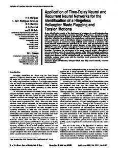
Figure 5: The response curves of system (39) with impulsive effects (𝛾 = 2.7556).
𝑘 ∈ 𝑍+ .
The matrices are given as follows: 𝐴=( 𝐶=(
0.1 0.1 0 0.2 0.1 0.1 0.1 0.1
),
0.02 0.1 ), 𝐵=( 0 −0.1
),
𝐶𝑘 = (
0.1 0 ̃= ( ), 𝐴 0 0 ̃= ( 𝐶
0 0.1 0 0.1
),
𝐵̃ = (
𝑐1 0 0 𝑐2
),
0.01 0 0
It is easy to see that 𝐾1 = 𝐿 1 = 0, 𝐾2 = 𝐿 2 = 0.5𝐼. We choose 𝑛𝑘 − 𝑛𝑘−1 = 5, and solving LMI (1) in Theorem 9, we get
0.1
𝑊1 = ( (40)
),
1 0.1 ̃=( ), 𝐷 0 1
𝑥(𝑛) = (𝑥1 (𝑛), 𝑥2 (𝑛))𝑇 , 𝑓(𝑥(𝑛)) = (𝑓(𝑥1 (𝑛)), 𝑓(𝑥2 (𝑛)))𝑇 , 𝑔(𝑥(𝑛 − 𝜏)) = (𝑔(𝑥1 (𝑛 − 𝜏)), 𝑔(𝑥2 (𝑛 − 𝜏)))𝑇 , 𝑓𝑖 (𝑠) = 𝑔𝑖 (𝑠) = tanh(𝑠), 𝜏 = 2.
0.5 0 0 0.1
),
0.2 0 𝑊2 = ( ). 0 0.2
(41)
By choosing 𝑐1 = 0.16, 𝑐2 = 0.15, 𝛼 = 0.21, 𝛽 = 0.14, and 𝜀 = 3.25, we get 𝛾 = 0.0256. Also by choosing 𝑐1 = 1.66 and 𝑐2 = 1.65, we derive 𝛾 = 2.7556. Whether 𝛾 = 0.0256 or 𝛾 = 2.7556, condition (2) of Theorem 9 always holds. Thus the trivial solution of system (39) is globally exponentially stable. Figure 3 depicts the state trajectories 𝑥1 (𝑛) and 𝑥2 (𝑛) of system (39) without impulsive effects. Figures 4 and 5 depict the state variables 𝑥1 (𝑛) and 𝑥2 (𝑛) with different impulsive effects, respectively.
8 Remark 13. In Example 1, compared with Figures 1 and 2, we get that impulse effects will make unstable system stable if conditions of Theorem 7 hold. Similarly, according to Example 2, uncertain systems with delay and impulse will also be stable if the conditions of Theorem 9 hold. Consequently, through two examples, we have the following results. On the one hand, when the original dynamic system is stable, we figure out feasible regions of impulses that can keep the stability property of the system. On the other hand, when the original dynamic system is unstable, we use impulses to stabilize it.
5. Conclusions In this paper, the stability of discrete-time impulsive delayed neural network with and without uncertainty has been investigated. Uncertain parameters take values in some intervals. By applying Lyapunov functions and Razumikhintype theorems, as well as linear matrix inequalities (LMIs), some new results for achieving exponential stability have been derived. Meanwhile, two examples together with their simulations have been presented to show the effectiveness and the advantage of the presented results.
Conflict of Interests The authors declare that there is no conflict of interests regarding the publication of this paper.
Acknowledgments This work was supported by the National Natural Science Foundation of Peoples Republic of China (Grants no. 61164004, no. 61473244, and no. 11402223), Natural Science Foundation of Xinjiang (Grant no. 2013211B06), Project Funded by China Postdoctoral Science Foundation (Grants no. 2013M540782 and no. 2014T70953), Natural Science Foundation of Xinjiang University (Grant no. BS120101), and Specialized Research Fund for the Doctoral Program of Higher Education (Grant no. 20136501120001).
References [1] H. Lu, R. Shen, and F.-L. Chung, “Global exponential convergence of Cohen-Grossberg neural networks with time delays,” IEEE Transactions on Neural Networks, vol. 16, no. 6, pp. 1694– 1696, 2005. [2] S. Guo and L. Huang, “Stability analysis of Cohen-Grossberg neural networks,” IEEE Transactions on Neural Networks, vol. 17, no. 1, pp. 106–117, 2006. [3] W. Su and Y. Chen, “Global robust stability criteria of stochastic Cohen-Grossberg neural networks with discrete and distributed time-varying delays,” Communications in Nonlinear Science and Numerical Simulation, vol. 14, no. 2, pp. 520–528, 2009. [4] W. Luo, S. Zhong, and J. Yang, “Global exponential stability of impulsive Cohen-Grossberg neural networks with delays,” Chaos, Solitons & Fractals, vol. 42, no. 2, pp. 1084–1091, 2009.
Discrete Dynamics in Nature and Society [5] Z. Orman, “New sufficient conditions for global stability of neutral-type neural networks with time delays,” Neurocomputing, vol. 97, pp. 141–148, 2012. [6] S. Mohamad, “Exponential stability in Hopfield-type neural networks with impulses,” Chaos, Solitons and Fractals, vol. 32, no. 2, pp. 456–467, 2007. [7] Z. Chen and J. Ruan, “Global dynamic analysis of general Cohen-Grossberg neural networks with impulse,” Chaos, Solitons and Fractals, vol. 32, no. 5, pp. 1830–1837, 2007. [8] Z. Chen and J. Ruan, “Global stability analysis of impulsive Cohen-Grossberg neural networks with delay,” Physics Letters A, vol. 345, no. 1–3, pp. 101–111, 2005. [9] Z. Yang and D. Xu, “Impulsive effects on stability of CohenGrossberg neural networks with variable delays,” Applied Mathematics and Computation, vol. 177, no. 1, pp. 63–78, 2006. [10] Q. Song and J. Zhang, “Global exponential stability of impulsive Cohen-Grossberg neural network with time-varying delays,” Nonlinear Analysis: Real World Applications, vol. 9, no. 2, pp. 500–510, 2008. [11] B. Liu and D. J. Hill, “Impulsive consensus for complex dynamical networks with nonidentical nodes and coupling timedelays,” SIAM Journal on Control and Optimization, vol. 49, no. 2, pp. 315–338, 2011. [12] Y. Shao, “Existence of exponential periodic attractor of BAM neural networks with time-varying delays and impulses,” Neurocomputing, vol. 93, pp. 1–9, 2012. [13] S. Mohamad and K. Gopalsamy, “Dynamics of a class of discrete-time neural networks and their continuous-time counterparts,” Mathematics and Computers in Simulation, vol. 53, no. 1-2, pp. 1–39, 2000. [14] W. Li, L. Pang, H. Su, and K. Wang, “Global stability for discrete Cohen-Grossberg neural networks with finite and infinite delays,” Applied Mathematics Letters, vol. 25, no. 12, pp. 2246–2251, 2012. [15] S. Mohamad and K. Gopalsamy, “Exponential stability of continuous-time and discrete-time cellular neural networks with delays,” Applied Mathematics and Computation, vol. 135, no. 1, pp. 17–38, 2003. [16] Z. Chen, D. Zhao, and X. Fu, “Discrete analogue of high-order periodic Cohen-Grossberg neural networks with delay,” Applied Mathematics and Computation, vol. 214, no. 1, pp. 210–217, 2009. [17] S. Wu, C. Li, X. Liao, and S. Duan, “Exponential stability of impulsive discrete systems with time delay and applications in stochastic neural networks: a Razumikhin approach,” Neurocomputing, vol. 82, pp. 29–36, 2012. [18] Y. Zhang, “Exponential stability analysis for discrete-time impulsive delay neural networks with and without uncertainty,” Journal of the Franklin Institute, vol. 350, no. 4, pp. 737–756, 2013. [19] Y. Sun, J. Cao, and Z. Wang, “Exponential synchronization of stochastic perturbed chaotic delayed neural networks,” Neurocomputing, vol. 70, no. 13–15, pp. 2477–2485, 2007. [20] S. Boyed, L. Ghaoui, E. Feron, and V. Balakrishnan, Linear Matrix Inequalities in System and Control Theory, SIAM, Philadelphia, Pa, USA, 1994. [21] Q. Song and J. Cao, “Dynamical behaviors of discrete-time fuzzy cellular neural networks with variable delays and impulses,” Journal of the Franklin Institute, vol. 345, no. 1, pp. 39–59, 2008. [22] S.-L. Wu, K.-L. Li, and J.-S. Zhang, “Exponential stability of discrete-time neural networks with delay and impulses,” Applied Mathematics and Computation, vol. 218, no. 12, pp. 6972–6986, 2012.
Discrete Dynamics in Nature and Society [23] Y. Li and C. Wang, “Existence and global exponential stability of equilibrium for discrete-time fuzzy BAM neural networks with variable delays and impulses,” Fuzzy Sets and Systems, vol. 217, pp. 62–79, 2013. [24] W. Xiong and J. Cao, “Global exponential stability of discretetime Cohen-Grossberg neural networks,” Neurocomputing, vol. 64, pp. 433–446, 2005. [25] M. Luo and S. Zhong, “Global dissipativity of uncertain discrete-time stochastic neural networks with time-varying delays,” Neurocomputing, vol. 85, pp. 20–28, 2012. [26] C. Li, S. Wu, G. G. Feng, and X. Liao, “Stabilizing effects of impulses in discrete-time delayed neural networks,” IEEE Transactions on Neural Networks, vol. 22, no. 2, pp. 323–329, 2011. [27] B. Liu and H. J. Marquez, “Uniform stability of discrete delay systems and synchronization of discrete delay dynamical networks via Razumikhin technique,” IEEE Transactions on Circuits and Systems. I. Regular Papers, vol. 55, no. 9, pp. 2795– 2805, 2008. [28] X. Li, “Existence and global exponential stability of periodic solution for delayed neural networks with impulsive and stochastic effects,” Neurocomputing, vol. 73, no. 4–6, pp. 749– 758, 2010. [29] L. Hou, G. Zong, and Y. Wu, “Robust exponential stability analysis of discrete-time switched Hopfield neural networks with time delay,” Nonlinear Analysis: Hybrid Systems, vol. 5, no. 3, pp. 525–534, 2011. [30] X.-L. Zhu, Y. Wang, and G.-H. Yang, “New delay-dependent stability results for discrete-time recurrent neural networks with time-varying delay,” Neurocomputing, vol. 72, no. 13–15, pp. 3376–3383, 2009. [31] L. Jarina Banu, P. Balasubramaniam, and K. Ratnavelu, “Robust stability analysis for discrete-time uncertain neural networks with leakage time-varying delay,” Neurocomputing, vol. 151, no. 2, pp. 808–816, 2015. [32] R. Samli, “A new delay-independent condition for global robust stability of neural networks with time delays,” Neural Networks, vol. 66, pp. 131–137, 2015.
9
Advances in
Operations Research Hindawi Publishing Corporation http://www.hindawi.com
Volume 2014
Advances in
Decision Sciences Hindawi Publishing Corporation http://www.hindawi.com
Volume 2014
Journal of
Applied Mathematics
Algebra
Hindawi Publishing Corporation http://www.hindawi.com
Hindawi Publishing Corporation http://www.hindawi.com
Volume 2014
Journal of
Probability and Statistics Volume 2014
The Scientific World Journal Hindawi Publishing Corporation http://www.hindawi.com
Hindawi Publishing Corporation http://www.hindawi.com
Volume 2014
International Journal of
Differential Equations Hindawi Publishing Corporation http://www.hindawi.com
Volume 2014
Volume 2014
Submit your manuscripts at http://www.hindawi.com International Journal of
Advances in
Combinatorics Hindawi Publishing Corporation http://www.hindawi.com
Mathematical Physics Hindawi Publishing Corporation http://www.hindawi.com
Volume 2014
Journal of
Complex Analysis Hindawi Publishing Corporation http://www.hindawi.com
Volume 2014
International Journal of Mathematics and Mathematical Sciences
Mathematical Problems in Engineering
Journal of
Mathematics Hindawi Publishing Corporation http://www.hindawi.com
Volume 2014
Hindawi Publishing Corporation http://www.hindawi.com
Volume 2014
Volume 2014
Hindawi Publishing Corporation http://www.hindawi.com
Volume 2014
Discrete Mathematics
Journal of
Volume 2014
Hindawi Publishing Corporation http://www.hindawi.com
Discrete Dynamics in Nature and Society
Journal of
Function Spaces Hindawi Publishing Corporation http://www.hindawi.com
Abstract and Applied Analysis
Volume 2014
Hindawi Publishing Corporation http://www.hindawi.com
Volume 2014
Hindawi Publishing Corporation http://www.hindawi.com
Volume 2014
International Journal of
Journal of
Stochastic Analysis
Optimization
Hindawi Publishing Corporation http://www.hindawi.com
Hindawi Publishing Corporation http://www.hindawi.com
Volume 2014
Volume 2014