verses of data are performed over abstract domains. The ap- plication of abstract ...... If there is one entry with non-expired lease, the space can decrease the ...
Abstraction of Parallel Uniform Processes with Data∗ Jun Pang, Jaco van de Pol, Miguel Valero Espada CWI, Department of Software Engineering, The Netherlands {pangjun,vdpol,miguel}@cwi.nl Abstract In practice, distributed systems are quite often composed by an arbitrarily large but finite number of processes that execute a similar program. Abstract interpretation is an effective technique to fight state explosion problems. In this paper, we propose a general framework for abstracting parallel composition of uniform processes with data, in the setting of a process algebraic language µCRL. We illustrate the feasibility of this technique by proposing two instances of the general framework and applying them to the verification of two systems.
1. Introduction In practice, distributed systems are quite often composed by an arbitrarily large but finite number of processes that execute a similar program. The parallel composition of a set of uniform processes with data always produces an exponentially growing state space, which limits the application of verification techniques such as model checking. Abstract interpretation [4] is an effective technique to fight the state explosion. It extracts program approximations by eliminating uninteresting information. Computations over concrete universes of data are performed over abstract domains. The application of abstract interpretation to the verification of systems is suitable since it allows to formally transform possibly infinite instances of specifications into smaller and finite ones. By loosing some information we can compute a desirable view of the analyzed system that preserves some interesting properties of the original. Algebraic approaches to the study of distributed systems focus on the manipulation of process descriptions. Process algebras, are well suited for the study of behavioral properties of distributed systems. The language µCRL [11] combines the process algebra ACP [2] with equational abstract ∗
Partially supported by PROGRESS, the embedded systems research program of the Dutch organization for Scientific Research NWO, the Dutch Ministry of Economic Affairs and the Technology Foundation STW, grants CES.5008 and CES.5009.
data types. To each µCRL specification there belongs a Labeled Transition System, in which the states are process terms and the edges are labeled with actions. Linear Process Equations (LPEs) [21] constitute a restricted class of µCRL specifications, in which the parallel composition and communication operators are removed. Algorithms have been developed to transform µCRL specifications into this linear format. In particular, Groote and van Wamel [12] derived an LPE for the parallel composition of an arbitrary but finite number of uniform processes with data. Recently, van de Pol and Valero Espada [19] developed a framework to generate modal abstract approximations from µCRL specifications. They introduced a new format for process specifications Modal Linear Process Equation (ModalLPE), in which every transition, labeled with a set of abstract actions, may lead to a set of abstract states. They used Modal-LPEs to characterize abstract interpretations of systems and to generate Modal Labeled Transition Systems (Modal-LTS), in which transitions may have two modalities may and must, that represent a double approximation (over and under) of the original system, and proved that the abstractions are sound for the full action-based µ-calculus. Considering a distributed system composed of an arbitrary but finite number of uniform processes with data, we develop a general framework and its formal requirements for safely abstracting the system by performing abstract interpretation of data, based on [12, 19]. Moreover, we present two abstraction patterns, which fulfill the requirements and can be embedded in the general framework. 1. Abstraction of process state: instead of keeping the state of each process, we only count the number of processes that are in a certain state. 2. Abstraction of the state counter: instead of storing the exact number of processes that are in a same state, we only consider some specific cases of the counter. Furthermore, we present a special abstraction schema for systems composed by indistinguishable processes, i.e., their behavior does not depend on their identity. We illustrate the feasibility of our technique by verifying a (simplified) distributed lift system [10] and a shared data space architec-
ture built over the JavaSpaces architecture [17]. For experiments we used the abstraction assistent [18] in the µCRL toolset [3]. Our approach can be used to verify large instances of distributed systems. Moreover, in combination with classical data abstraction, we can generalize the results to any instance of parameters of the system. In this extended abstract, we omit the proofs for all the theorems. Interested readers can find them at: http://www.cwi.nl/˜miguel/abstraction/
Related work. The Parameterized model checking problem, which is in general not decidable [1], has been addressed in several works using different approaches. Abstraction techniques for model checking are sound but incomplete, and need human creative interactions in order to select the appropriate abstractions. The closest to ours are [15, 20]. Ip and Dill [15] used a special data type to represent process identities and perform an abstraction that maps the processes that are in a certain state to the values {zero, more, zero or more}. The work by Pong and Dubois [20] follows the same idea but needs more user interaction in order to define the abstract behavior of the abstracted processes. An improvement of our approach with respect to theirs is that we can deal with both safety and liveness properties. Moreover, we do not give a fixed abstraction mapping but a general pattern that can be instantiated with different abstraction relations. The parallel composition of processes is automatically translated to a required form, therefore the user only needs to define the desired abstractions. Liveness for parametrized systems was already addressed in [16]. To use this approach, one has to define safe acceleration schemes in order to infer liveness properties. Automated and complete techniques, e.g. the one proposed by Emerson and Kahlon for Snoopy Cache Coherence Protocols [7], are restricted to a particular set of systems. Other sound but incomplete methods use, for example, automatically inductive invariants generated from small instances of a system that hold in every larger instance of it. Another approach is based on a cutoff theorem, which has to be found and proved in order to generalize the verification result (see a.o. [6]). This paper is organized as follows: Some basic definitions and a short introduction to modal abstraction in µCRL are given in Section 2. The general framework for linearizing and abstracting of parallel uniform processes with data is proposed in Section 3. Section 4 presents two abstraction patterns, and Section 5 applies these two patterns to a particular set of systems where processes are indistinguishable. We perform two case studies in Section 6 and conclude the paper in Section 7.
2. Preliminaries 2.1. Transition Systems The semantics of a system can be captured by a Labeled Transition System (LTS). An LTS consists of a possibly ina finite set of transitions s → s′ , denoting that the state s can ′ evolve into the state s by the execution of an action a. To model abstractions we use a different structure that allows to represent approximations of the concrete system in a more suitable way. In a Modal Labeled Transition System (Modal-LTS), transitions have two modalities may and must which denote the possible and necessary steps in the refinements. This concept was introduced by Larsen and Thomsen [14]. The formal definition extends the definition of LTSs by considering the two modalities. From a concrete system described by an LTS we can generate an abstraction of it by relating concrete states and action labels with abstract ones. We use a classical abstraction framework based on Galois Connections between domains, introduced in the late seventies by Cousot and Cousot [4], see also [5]. Given the abstraction relation, we construct a double approximation of the concrete system using a Modal-LTS. The may-transitions correspond to an over-approximation of the original and the must ones to an under-approximation. In [19], we have presented the complete formal framework for performing abstractions, now we give an example to introduce the basic intuition1 : B Concrete States Abstract States
b A a
b a
a a
a
a
Concrete Transitions Abstract May Transitions Abstract Must Transitions
C a
b b b
b
If all concrete states related to an abstract state S have a transition to a concrete state related to an abstract state S ′ , then there is a must transition between S and S ′ . Therefore, a in Figure 2.1, we have the abstract must transition B → C. If there is some concrete state related to an abstract state S with a transition to another state related to an abstract state S ′ , then there is a may transition between S and S ′ . In Figure 2.1, these abstract transitions are marked by the dashed arrows. Whenever there is a must transition, there is also a may one, note that we do not explicitly draw such cases. Since the abstraction of a system preserves some information of the original one, the idea is to prove properties on 1
The example is simplified by leaving out abstraction of labels.
the abstract and then to infer the result for the original. To express properties about systems, we adapt the highly expressive temporal logic (action-based) µ-calculus [13]. The satisfaction and/or refutation of formulas built over the full µ-calculus is preserved/reflected in the abstract systems. In the above example, we can prove a liveness property that states that from the initial state we can do an atransition (hai T ) because in the abstract system there is a must transition from A, so A necessarily satisfies hai T . Furthermore, we can refute that from the initial state it is possible to do a c-transition (hci T ) because there is no abstract may c-transition from A.
2.2. µCRL µCRL [11] is a formal language for specifying protocols and distributed systems in an algebraic style. A µCRL specification consists of two parts: one part specifies the data types, the other part specifies the processes. We assume the existence of the data types: booleans and naturals, denoted by Bool and Nat with their standard functions. Moreover, for every data type we assume the existence of the equality predicate. The specification of a process is constructed from action names, recursion variables and process algebraic operators. Actions and recursion variables carry zero or more data parameters. There are two predefined actions in µCRL: δ represents deadlock, and τ a hidden action. These two actions never carry data parameters. Processes are represented by process terms, which describe the order in which the actions from a set Act may happen. A process term consists of action names and recursion variables combined by process algebraic operators. p·q denotes sequential composition and p + q non-deterministic P choice, summation d:D p(d) provides the possibly infinite choice over a data type D, and the conditional construct p�b�q with b a data term of data type Bool behaves as p if b and as q if ¬b. Parallel composition p k q interleaves the actions of p and q; moreover, actions from p and q may also synchronize to a communication action. The syntax and semantics of µCRL are given in [11].
2.3. Linearization and Abstraction of µCRL Specifications Linearization. A Linear Process Equation (LPE) is a single equation consisting of actions, summations, sequential compositions and conditional constructs. In particular, an LPE does not contain any communication and parallel operators. In essence an LPE is a vector of data parameters together with a list of condition, action and effect triples, describing when an action may happen and what is its effect on the vector of data parameters. Each µCRL specification
that does not include successful termination can be transformed into an LPE [21]. Definition 2.1 A Linear Process Equation is a µCRL specification of the form X(d : D) =
XX
ai (fi (d, ei )).X(gi (d, ei )) � ci (d, ei ) � δ
i∈I ei :Ei
where ci : D × Ei → Bool, fi : D × Ei → Di , gi : D × Ei → D, and ai is an action label with data parameters of type Di . The LPE expresses that state d can perform, for all ei : Ei , an action ai (fi (d, ei )) to end up in state gi (d, ei ), under the condition that ci (d, ei ) is true. To every LPE corresponds a Labeled Transition System, in which process states are represented by the nodes and actions by transition labels. Abstraction. To generate a “safe” abstraction of a µCRL specification we first give the abstraction relation between the data domains, concrete and abstract, and then we interpret the concrete system over the abstract domain. Let absD be the abstract domain, and let us consider the relation between concrete and abstract domains is given by an arbitrary mapping H : D → absD 2 . To generate an abstract approximation, we first transform the original specification to a new format, called Modal Linear Process Equation, then we extract the corresponding Modal-LTS from it. Before introducing the definition of the Modal-LPE, we present a simple example. Let us consider a concrete specification that uses integers. Then, if we abstract the integers to their sign, i.e., {neg, zero, pos}, we need to provide abstract definitions of the functions to manipulate them. For example, the abstract successor of neg can be either neg or pos, the abstract successor of zero is pos and the abstract successor of pos is always pos. In the first definition, we see that abstract function may add more non-determinism. To capture this feature, we use sets of values, i.e., absSucc(neg) = {neg, zero}. A Modal-LPE is similar to an LPE, the difference is that the state is represented by power sets of abstract values and for every i: Ci returns a non-empty set of booleans, Gi a non-empty set of states and Fi a non-empty set of action parameters. Definition 2.2 A Modal Linear Process Equation is a µCRL specification of the form X(aD : P(absD)) =
P
i∈I
P
ei :Ei
ai (Fi (aD, ei )).
X(Gi (aD, ei )) � Ci (aD, ei ) � δ 2
In fact, H may be an arbitrary relation, but for simplicity we assume that it is a mapping.
where Ci : P(absD) × Ei → P(Bool), Fi : P(absD) × Ei → P(absDi ), and Gi : P(absD) × Ei → P(absD). Concrete LPEs are automatically abstracted using the abstraction assistant for µCRL specifications [18]. As the result of the syntactic transformation, we obtain a Modal-LPE in which concrete function symbols f, appearing in the data terms fi , gi , and ci of the original specification, are replaced by abstract counterparts absF, resulting in the corresponding abstract terms Fi , Gi , and Ci . In order to generate a Modal-LTS the user has to provide the relation between concrete and abstract domains H and the definition of the abstract function symbols that form part of the abstract Modal-LPE generated by the tool. The semantics of Modal-LPEs follow these rules: A
• S →must S ′ if and only if there exists i ∈ I and e ∈ Ei such that F ∈ / Ci (S, e), A = a(Fi (S, e)) and S ′ = Gi (S, e) A
• S →may S ′ if there exists i ∈ I and e ∈ Ei such that T ∈ Ci (S, e), and A = a(Fi (S, e)) and S ′ = Gi (S, e) A Modal-LTS, generated from an abstract Modal-LPE, is a safe approximation of the original system, if the abstract functions that appear in the data terms of the Modal-LPE satisfy a formal requirement in relation with their concrete counterparts. Every pair of functions (f, absF), in which f : X → Y (X is a vector of sorts) and absF : absX → P(absY), has to satisfy: • ∀ x : X. H(f(x)) ∈ absF(H(x)) We assume that the abstract function of the boolean sort is the identity. We also remark that all functions are considered to apply point-wisely to sets. In the next section, we present the general framework to specify the parallel composition of uniform processes and the abstraction of them by following the ideas presented in this section.
3. Linearization and Abstraction of Parallel Uniform Processes Linearization. We use µCRL to specify systems composed by an arbitrary number of uniform processes. We assume that the processes are loosely coupled, i.e., they do not communicate directly with each other.3 However, we allow them to communicate with external processes that may play the role of networks or coordination architectures. Uniform processes share the same specification, i.e., they are syntactically the same. This does not mean that their behavior
is equal for all of them. Every processes is uniquely identified, by a natural number k, and its behavior may be determined by its identity. From now on, we assume that the uniform processes share the following linear form (see Definition 2.1): P (k : Nat, d : D) = P P i∈I
This requirement is not necessary, it is just to simplify the development.
ai (fi (k, d, ei )).
P (k, gi (k, d, ei )) � ci (k, d, ei ) � δ
This linear form makes no restriction on the specification of the processes. For a process P (k, d), k is the identity and d the data parameter of some arbitrary data type D representing the state of the process.4 We assume the existence of a global constant N > 1 denoting the number of uniform processes, therefore k is in the range {0, . . . , N − 1 }. Groote and van Wamel [12] defined an equation that models the parallel composition of N such processes, it uses a data type DTable to store the values of parameters d of each process. It defines tables indexed by natural numbers, and each element has the data type D. Based on their definitions, we specify a different representation that is more appropriate for performing abstractions. Let K denote the set {0, . . . , N − 1}. The data type DTable has the signature of K → D. Each table is a function from K to D. Thus, a process with identity k only has one state in a table. Furthermore, we define update as a function to update the old value e of process P (k) with d, test a function to check whether the specified position and data are in the table. update : test :
K × D × D × DTable → DTable K × D × DTable → Bool
The defining equations are: update (k, d, e, dt) =def test (k, d, dt) =def
dt [ k := d ] dt(k ) = d
The argument e of update represents the old value of the process k, it is not necessary for the definitions of concrete linear systems, however we will see that it is helpful to define abstraction patterns. Let dk be the initial value of the process k and dt be initially defined as dt (k ) = dk for all k ∈ K, then: Theorem 3.1 The system P (0, d0 ) || P (1, d1 ) || · · · || P (N − 1, dN −1 ) is strongly bisimilar to Q(dt), where Q is an LPE of the form: 4
3
ei :Ei
Typically processes have a vector of parameters, using pairing and projections we can easily see that the use of a single parameter d is not an essential limitation.
Q(dt : DTable) = P P P i∈I
k:Nat
d:D
P
ei :Ei
ai (fi (k, d, ei )).
Q(update(k, gi (k, d, ei ), d, dt))
�test (k, d, dt) ∧ ci (k, d, ei ) ∧ k < N � δ
Theorem 3.1 states that any parallel composition of uniform processes can be encoded using an LPE and a data type DTable. Instead of the condition test, Groote and van Wamel used a function get to access the state of the processes. Both approaches are equivalent for defining concrete systems, in which every process is in only one state. However, our approach minimizes the extra non-determinism added by the abstractions that do not allow to determine the exact state of the processes. Abstraction. Now we present an abstraction framework for an LPE in Theorem 3.1. It is composed by some definitions and requirements that any particular instance of abstraction must fulfill. To perform an abstraction it is needed to specify a mapping H from concrete tables DTable to abstract ones absDTable. Furthermore, the concrete linear form is symbolically abstracted to the following Modal-LPE (see Definition 2.2): absQ(absDt : P(absDTable)) = P P P P i:I
k:Nat
d:D
ei :Ei
ai (fi (k, d, ei )).
absQ(absUpdate (k, gi (k, d, ei ), d, absDt )) �absTest (k, d, absDt ) ∧ ci (k, d, ei ) ∧ k < N � δ
absQ is the abstract version of the process defined in Theorem 3.1, it gets as a parameter the abstract specification absDTable, that is initialized by the abstraction of the concrete initial table, i.e., H(dt), and can be accessed with the functions absUpdate and absTest, which have the following signatures: absU pdate : K × D × D × absDT able → P(absDT able) absT est : K × D × absDT able → P(Bool)
Recall that all the functions point-wisely apply to sets of values. The function symbols appearing in the data terms are: absTest , ∧, ci , 1). To perform this abstraction we define an abstract counter absCount by specifying a new mapping Hc : Count → absCount . The data type absCount has three values: zero, some and all. Together, we define two functions absSucc, absPred : absCount → P(absCount ) to increase and decrease an abstract counter.
Hc (c) =def absSucc(zero) =def absP red(zero) =def absSucc(some) =def absP red(some) =def absSucc(all) =def absP red(all) =def
8 if c = N < all some if 0 < c < N : zero if c = 0 {some} {zero} {some, all} {zero, some} {all} {some}
The function absMatch is used to check whether a process is in a certain state, based on the information of the abstract counter. It corresponds to the function match for Count. absM atch(zero) =def absM atch(some) =def absM atch(all) =def
{F} {T, F} {T}
In our second instance of the general framework, we redefine absDTable as a data type with the signature D →
absCount . Accordingly, absDt(d) expresses the abstract number of processes which are in state d. absUpdate is a function to update the number of processes in one state. The definition of the new functions are as the ones defined in the previous section, the only difference is that we replace the concrete functions for the counter by abstract ones: absT est(k, d, absDt) =def absM atch(absDt(d)) Succ(absDt, d) =def absDt[d := absSucc(absDt(d))] P red(absDt, d) =def absDt[d := absP red(absDt(d))] absU pdate(k, d, e, absDt) =def {Succ(P red(absDt, e), d))}
The new table is a more abstract version of the previous one. The abstract mapping Htc : DT able → absDT able, is the combination of the mappings Ht and Hc : Htc (dt)(d) =def Hc (Ht (dt)(d))
Theorem 4.2 The abstract table with abstract counters constructed using the mapping Htc , defines a safe abstraction. Considering the result of Theorem 4.1, the two safety requirements for the functions absTest and absUpdate reduce to prove that ∀c : Count the following conditions hold: Hc (Succ(c)) ∈ Hc (P red(c)) ∈ match(c) ⊆
absSucc(Hc (c)) absP red(Hc(c)) absM atch(Hc (c))
This pattern is more abstract than the previous, therefore it will preserve less information. We remark, again, that the abstraction patterns are just examples of instances that match the general framework provided in Section 3. Depending on the system other values for the abstract counter may be selected, for example the domains {zero, one, more} or {zero, more, zero or more} used in Ip and Dill’s work [15] are easily embedded in our framework. This abstraction pattern may be also combined with the previous one by only abstracting the counters related to some specific states and leaving the others as natural counters.
5. Linearization and Abstraction of Parallel Identical Processes Linearization. Section 3 was dedicated to the linearization and abstraction of uniform processes. We have defined uniform processes as the ones that share the same specification, i.e., they are syntactically the same. Each process has assigned an unique identity. Even if two processes are syntactically the same, their behavior may be different because of their identity.
We consider a particular case of uniform processes which are indistinguishable. We call this class of processes identical. The behavior of each process does not depend on its own identity k. They share the following linear form: P (d : D) =
P
i∈I
P
ei :Ei
ai (fi (d, ei )).P (gi (d, ei ))
�ci (d, ei ) � δ
Given two identical processes pi and pj that are in the same state d. If a condition c is true for pi , then it is also true for pj . Furthermore, they can execute the same action to end in the same new state. If processes are identical then the mapping of Section 4.1 does not loose information. Therefore, the concrete system is composed by a table that stores the number of processes that are in a certain state. We redefine the concrete table DTable =def D → Count . So dt(d) states the number of processes in a certain state d. Accordingly, we redefine the functions update and test. update : test :
D × D × DTable → DTable D × DTable → Bool
The defining equations are:
T if dt(d) > 0 F if dt(d) = 0 dt[d := Succ(dt(d ))] dt[d := Pred (dt(d ))] Succ(P red(absDt, e), d))
test (d, dt) =def Succ(dt, d) =def Pred (dt, d) =def update(d, e, dt) =def
Let ni the number of identical processes that are initially in the state di , and dt be defined as dt (di ) = ni , then we have the following theorem: Theorem 5.1 P (d0 ) || P (d1 ) || · · · || P (dN −1 ) is strongly bisimilar to Q(dt), which is an LPE of the following form: Q(dt : DTable) =
P
i∈I
P
d:D
P
ei :Ei
6. Applications 6.1. JavaSpaces JavaSpaces [9] is a coordination architecture that implements a shared repository that external agents can use to communicate by sharing objects. It provides extra support for implementing reliable applications. Systems may use transactions, a notification mechanism and timeouts on resource allocation. We focus on a characteristic sort of applications that coordination architectures, such as JavaSpaces, can easily implement. The idea is to accomplish a computationally intensive problem by breaking it into a number of smaller tasks that can be executed in parallel. In particular, we consider a simple example composed by three different types of components: • Producer: It writes new entries into the space. We can think the producer as an acquisition unit that generates a continuous flux of data that have to be processed. We mark the unprocessed entries as being of type A. • Transformer: It retrieves entries of type A, performs some computation and writes a transformed entry into the shared repository. The processed entry is of type B. • Consumer: It takes the processed information from the space, and uses the result of the computations. A real life example that can match our model is, for example, a radar-monitor system. The radar introduces packets of different measurements taken from an external moving agent. Transformers process the measures by computing predictions of future moves of the investigated agent. The monitor displays the results of the process. In general, we would like to have several transformers making calculations at the same time in order to accelerate the display of the results. Next figure presents an overview of the system.
ai (fi (d, ei )).
Q(update(gi (d, ei ), d, dt)) �test (d, dt) ∧ ci (d, ei ) � δ
Instead of storing the state of every process, we have used a counter representing the number of processes that are in a certain state and we have proved that both representations are equivalent (are strongly bisimilar). Abstraction. In order to abstract the system with identical processes, we can trivially adapt the definitions given for the case of uniform processes. In this case the abstraction would consist of abstraction of the counters, therefore, one may use, for example, the pattern provided in Section 4.2, in which the counter is abstracted to some symbolic values that determine the abstract number of processes that are in a certain state.
1 0 0 1
write
00P 11 1 0 0 1 0 1 0 1
A entry
1 0 01 1 0 0 1 take
B entry
T
write
1 0 0 1
take
11 C 00
0 1 1 0 1 0 0 1 take
write
11 00 1 0 0 1 T
In previous work [17], we developed a formal specification of JavaSpaces written in µCRL. The specification is not trivial and it captures the main features of the original architecture. It is composed by more than 500 lines of code. Below we present the µCRL specification of the three types of components. The complete concrete system is defined by the parallel composition of the space, the producer, the consumer, and N Transformers process.
proc Producer = write(A, timeout) .Producer proc Consumer = take(typeB) .TakeReturn(typeB, B) .Consumer
proc Transformer = take(typeA) .TakeReturn(typeA, A) .write(B, timeout) .Transformer
The Write action takes as arguments: the entry to add into the space and a lease, i.e., the time the entry is allowed to stay in the space before being automatically removed. Take actions are destructive reads, and are executed by two synchronous operations, first the space receives the request and then it returns the value. Take actions get as arguments the template used to select the desired entry. When there is an entry in the space that matches some request the space returns the desired value. The space only accepts a maximum number of queries active at the same time, we assume that this number is big enough for the needs of our system. The space makes the best effort in order to deliver the entries, i.e., it does not remove any entry that has a matching query. One basic requirement to check is that the system no matter what happens, keeps progressing. In other words that it will not deadlock. If the capacity of the space is bounded and the entries are never eliminated (infinite timeout), the system may arrive to a deadlock state. Let us consider a finite instance of the system with one single Transformer and the size of the space equals to 2. The following sequence of steps: 1) Producer writes A, 2) Producer writes A, 3) transformer takes A, 4) Produces writes A, leads to a deadlock since the space is full and the transformer cannot write a B entry, the producer cannot write any new entry either and the consumer cannot retrieve any B entry to free space. If the space is unbounded this problem will not arise since both producer and transformer can always write. But this solution is not realistic therefore we add a timeout to the entries which will allow the space to free some place for new incoming entries. In principle, using timeouts, there should not be any deadlock in the system, because in any state one of the following actions is possible: • If it is not full then the producer can Write. • If there is some A entry in the space, Transformers that are waiting for an entry can take it, (similar for B). • If there is one expired entry, i.e., its lease equals to 0, and no process is requiring it, then the space can remove the entry. • If there is one entry with non-expired lease, the space can decrease the timeout of the entry. Looking at the Transformer µCRL code, we see that they are identical, they do not use any identification number
therefore we can use the pattern presented in Section 5. Moreover, we can abstract it by doing an abstraction to the counters of the number of processes that are in one state, as presented in the pattern of Section 4.2. However, it is important to capture the idea that after every take action there should be exactly one return operation (TakeReturn). Therefore, we abstract all counters but the one that determines the number of processes that are waiting for an entry. The absence of deadlock may be expressed using the action based µ-calculus with modalities as follows: νX.( h ′ . ∗must .∗′ i true ∧ [ ′ . ∗may .∗′ ] X) The formula states that from every state that may be reached there is an out-going must transition. The property can be proved using the CADP toolset [8]. Below, we present a table with the sizes of the state spaces for different instances of the system. We compare three cases: • The concrete system represented with the standard representation of parallel processes (denoted by Crt). • The concrete system given in the linear form proposed in the equation of Theorem 5.1 (denoted by Crt Lin). • The abstract version of the last case (denoted by Abs). The table shows how the standard representation of parallel processes can not deal with big instances of the system. However, our proposed format can, because it eliminates symmetries of the interleavings. Moreover, with the abstraction we can reduce even more the size of the systems. It is possible to handle instances with more than 100 parallel processes. In order to generalize the model checking problem to an arbitrary number of processes, we would have to abstract also some parts of the JavaSpaces processes, more precisely, we would have to abstract the maximum number of active queries. Crt 5T 6T 7T 8T
States 15,135 49,560 161,097 520,494
Crt Lin 10T 20T 40T 80T
States 4,663 25,828 267,302 1,193,830
Abs 10T 20T 40T 80T 100T
States 3,858 12,093 42,171 156,759 241,269
This example shows that the proposed framework is suitable for verifying liveness properties. Many typical JavaSpaces applications follow the schema of the example, therefore they can easily be analyzed following our methodology.
6.2. A Distributed System for Lifting Trucks A real-life distributed system for lifting trucks (lorries, railway carriages, buses and other vehicles), which was designed and implemented by a Dutch company, was analyzed in µCRL together with CADP by Groote et al. [10]. The system consists of a number of lifts; each lift supports one wheel of the truck that is being lifted and has its
own micro-controller. On each lift there are some buttons that control its movement. The micro-controllers of the different lifts belonging to a system are connected to a ‘cyclical’ CAN (Controller Area Network). The formal analysis of the system discovered some errors in the original specification and helped to build a refined version of the incorrect implementation. The new specification could be proved correct for small instances of the system (at most 5 lifts). In this section, we are going to extend the analysis of some requirements for an arbitrary number. For this purpose, we first give a simplified version of the original specification that removes some non-relevant details, then we apply the previously introduced techniques (see Section 4.1 and Section 4.2). If the up button of a certain lift is pressed, all the lifts of the system should go up. The system has to assure that all lifts move simultaneously to the same direction. Lifts are programmed in such a way that during normal operation, they take turns to claim the bus. To achieve this orderly usage of the CAN bus, each lift must know its position in the network. Furthermore, in order to be able to find out whether all lifts are in the same state, each lift must know how many lifts there are in the network. Initially, all lifts are in a standby state. The state of a lift is changed if its up button is pressed. Then it will send an up message to the bus. Other lifts change their state according to the messages they receive, and when it is their turn to use the bus they broadcast a message according to their state. These messages are received by all the other lifts, and the lift where a button is pressed will count them. When it counts enough state messages and it gets the turn to use the bus, it will broadcast a move message, after which all the lifts will synchronously move. The state of each lift is the vector composed by: the identifier of the lift, which determines the order to claim the bus, the current state of the lift and a counter for synchronized lifts which ranges from 0 to N . The behavior of the lifts also depends on the passing messages, which are composed by: the identity, the state of the sender of the last message and a boolean specifying when the up-button was pressed. The complete system is composed by the parallel composition of the N lifts and the process that models the CAN bus. In order to create an abstraction that proves properties for an arbitrary number of lifts, we have to combine the abstraction of processes as proposed in this paper with classical data abstraction. Therefore, we first abstract all the parameters and local variables that depend on N . Then, we see that the behavior of the lifts depends on the process identifier so we have to use the abstraction pattern for uniform processes. Therefore, we construct the abstract table with abstract counters for every state using the abstraction pattern in Section 4.2. We have built such abstraction using the abstraction as-
sistant for µCRL specifications. The result of the abstraction is a Modal-LTS. We see below the comparison between the abstract result and some concrete instances. System Crt 5 Lifts Crt 6 Lifts Crt 7 Lifts Crt 8 Lifts Abs N Lifts
States 2,751 10,011 33,031 101,255 1341
Formally, we express a correctness criterion by the following safety property: [ true ∗ . ′ movemay ′ . NOTUP ∗ . ′ movemay ′ ]false Here NOTUP abbreviates (′ . ∗may . ∗′ ∧¬ ′ upmay ′ ), representing any may-step except upmay . Basically, the formula states that after a movement of the lift system, a button should be pressed in order to let the system move again. The safety formula is satisfied by the abstract system therefore we can infer its satisfaction to all instances of the concrete system. In this example we have seen that in some cases the abstraction patterns together with regular data abstraction may be used to generalize the model checking problem to an arbitrary number of uniform components. However the behavior of the lift system is strongly dependent of the identities of the lifts which implies that using the given patterns its abstraction will not preserve many liveness properties.
7. Conclusion We have presented a generic linearization and abstraction framework for algebraic specifications of systems composed by processes that execute a similar program. The framework is composed by a flexible set of definitions and formal requirements that may be instantiated with different abstraction schemes. Moreover, we have provided two different abstraction patterns that can be applied in a fully automated way. The suitability of the patterns has been proved by applying them to the verification of two distributed applications. Moreover, we have shown that, in some cases, the abstractions can still be used to verify liveness as well as safety properties. In Section 3, we have assumed that the uniform processes in parallel do not communicate between each other but with external processes. To generalize the framework for any kind of processes, we have to extend definitions of the linear equations by allowing communications via internal actions. The abstraction results will apply to the new definitions with no further change.
References [1] K.R. Apt and D. Kozen. Limits for automatic verification of finite-state concurrent systems. IPL, 22(6):307-309, 1986. [2] J.A. Bergstra and and J.W. Klop. Algebra of communicating processes with abstraction. TCS, 77–121, 1985. [3] S.C.C. Blom, W.J. Fokkink, J.F. Groote, I.A. van Langevelde, B. Lisser, and J.C. van de Pol. µCRL: A toolset for analysing algebraic specifications. In Proc. CAV’01, LNCS 2102, pp. 250–254. Springer, 2001. [4] P. Cousot and R. Cousot. Abstract interpretation: A unified lattice model for static analysis of programs by construction of approximation of fixed points. In Proc. POPL’77, pp. 238252. ACM, 1977. [5] D. Dams. Abstract Interpretation and Partition Refinement for Model Checking. PhD thesis, Eindhoven University of Technology, 1996. [6] E.A. Emerson and V. Kahlon. Reducing model checking of the many to the few. In Proc. CADE’00, LNCS 1831, pp. 236-254. Springer, 2000. [7] E.A. Emerson and V. Kahlon. Rapid parameterized model checking of snoopy cache coherence protocols. In Proc. TACAS’03, LNCS 2619, pp. 144-159. Springer, 2003. [8] J.-C. Fernandez, H. Garavel, A. Kerbrat, L. Mounier, R. Mateescu, and M. Sighireanu. CADP – a protocol validation and verification toolbox. In Proc. CAV’97, LNCS 1102, pp. 437–440. Springer, 1997. [9] E. Freeman, S. Hupfer and K. Arnold. JavaSpaces Principles, Patterns, and Practice. Addison-Wesley, 1999. [10] J.F. Groote, J. Pang, and A.G. Wouters. Analysis of a distributed system for lifting trucks. JLAP, 56(1-2):21-56, 2003. [11] J.F. Groote and A. Ponse. The syntax and semantics of µCRL. In Proc. 1st Workshop on ACP, Workshops in Computing Series, pp. 26–62. Springer, 1994. [12] J.F. Groote and J.J. van Wamel. The parallel composition of uniform processes with data. TCS, 266(1-2): 65-75, 2001. [13] D. Kozen. Results on the propositional µ-calculus. In Proc. ICALP’82, LNCS 140, pp. 348-359. Springer, 1982. [14] K.G. Larsen and B. Thomsen. A modal process logic. In Proc. LICS’88, pp. 203-210. IEEE CS, 1988. [15] C.N. Ip and D.L. Dill. Verifying systems with replicated components in Murφ. In Proc. CAV’96, LNCS 1102, pp. 147-158. Springer, 1996. [16] A. Pnueli and E. Shahar. Liveness and acceleration in parameterized verification. In Proc. CAV’00, LNCS 1855, pp. 328-343. Springer, 2000. [17] J.C. van de Pol and M. Valero Espada. Formal specification of JavaspacesTM architecture using µCRL. In Proc. COORDINATION’02, LNCS 2315, pp. 274–290. Springer, 2002. [18] J.C. van de Pol and M. Valero Espada. An Abstract Interpretation Toolkit for µCRL. Under Submission. [19] J.C. van de Pol and M. Valero Espada. Modal abstractions in µCRL. In Proc. AMAST’04, LNCS. Springer, 2004. To appear. [20] F. Pong and M. Dubois. A new approach for the verification of cache coherence protocols. IEEE TPDS, 6(8):773-787, 1995.
[21] Y.S. Usenko. Linearization in µCRL. PhD thesis, Eindhoven University, 2002.