Accelerating adiabatic quantum transfer for three-level $\Lambda ...

Accelerating adiabatic quantum transfer for three-level Λ-type structure systems via picture transformation Yi-Hao Kang1,2, Qi-Cheng Wu1,2 , Ye-Hong Chen1,2 , Zhi-Cheng Shi1,2 , Jie Song3 , and Yan Xia1,2,∗

arXiv:1703.01753v1 [quant-ph] 6 Mar 2017

1 Department

of Physics, Fuzhou University, Fuzhou 350116, China

2 Fujian

Key Laboratory of Quantum Information and

Quantum Optics (Fuzhou University), Fuzhou 350116, China 3 Department

of Physics, Harbin Institute of Technology, Harbin 150001, China

In this paper, we investigate the quantum transfer for the system with threelevel Λ-type structure, and construct a shortcut to the adiabatic passage via picture transformation to speed up the evolution. We can design the pulses directly without any additional couplings. Moreover, by choosing suitable control parameters, the Rabi frequencies of pulses can be expressed by the linear superpositions of Gaussian functions, which could be easily realized in experiments. Compared with the previous works using the stimulated Raman adiabatic passage, the quantum transfer can be significantly accelerated with the present scheme. PACS numbers: 03.67. Hk, 03.65. Ud Keywords: Shortcut to adiabatic passage; Picture transformation; Three-level Λ-type system

I.

INTRODUCTION

The three-level Λ-type system is known as a very important model in quantum information processing (QIP). Many quantum information tasks, such as the preparations of entanglement and the operations of various quantum gates, can be implemented in physical systems which are equivalent or approximately equivalent to three-level systems with Λ-type structures [1–16]. It is universally known that, to manipulate states of a three-level quantum system with electromagnetic field, there exists two typical methods, the π-pulse [17, 18] and the adiabatic passage [19–23]. These two methods hold their own advantages, ∗

E-mail: [email protected]

2 but both reveal their shortcomings. The π-pulse allows physical systems evolve quickly, but the pulses should be controlled very accurately, which bring challenges to experiments in some cases. On the other hand, the adiabatic passage is famous for its robustness against the imperfect operations and the deviations of the control parameters, but badly limits the evolution speed of the systems, which makes the systems more sensitive to some kinds of noise and decoherence factors. For the sake of both high evolution speed and robustness, a new technique named “Shortcuts to adiabatic passage” (STAP) [24–33] has been proposed. The STAP suggests the system evolving in a controllable nonadiabatic way, so that the adiabatic condition, which limits the evolution speed of the system, can be abandoned. Besides, when the boundary condition of the control parameters is well designed, the STAP is also robust against the imperfect operations and the deviations of the control parameters. Since the STAP combines the advantages of both the π-pulse and the adiabatic passage, it has attracted many interests of researches in different fields [34–56]. For example, Torrontegui et al. [41] have used STAP to transport Bose-Einstein condensates. Ruschhaupt et al. [43] have achieved a population inversion in a two-level quantum system with STAP. Among these schemes [24–56], the method named “transitionless quantum driving” (TQD) (also known as the “counterdiabatic driving”) [24–26, 55, 56] is one of the famous methods for constructing STAP, whose idea is to cancel the nonadiabatic transitions between the eigenstates for the original Hamiltonian of the system by adding “counterdiabatic” (CD) terms. The CD terms can be calculated easily, and their mathematic expressions are usually not too complex. For example, Demirplak et al. [24] have first used counterdiabatic fields to accelerate adiabatic passages, and shown that a population transfer between molecular states could be perfectly achieved, which is a pioneering work of STAP. Moreover, Du et al. [55] have experimentally shown that TQD could be used to design pulses to construct STAP for cold atoms. Furthermore, TQD has also be exploited by An et al. [56] to experimentally realize trapped-ion displacement in phase space. However, the CD terms sometimes play the roles as the additional couplings which are hard to be realized in real experiments. For example, it is indicated in many previous schemes [31, 57–59] that, for a three-level Λ-type atom, the CD terms are the special one-photon 1-3 pulse (the microwave field), which bring troubles to the experimental realization. To overcome the difficulties of TQD, many interesting schemes [60–73] have been put forward. For example, Ib´an ˜ ez et al. [66, 67] have pointed out that a sequence of shortcuts

3 to adiabaticity can be built with similar way of TQD via iterative interaction pictures. Subsequently, this method was used in a three-level system with Λ-type structure by Song et al. [68]. They have shown that the difficulties of TQD can be overcome, and the STAP can be constructed by adjusting the Rabi frequencies of pulses in original Hamiltonian, so the additional couplings are unnecessary. Chen et al. [71] have also come up with an interesting idea to construct an experimentally feasible Hamiltonian for a three-level system by using multi-mode driving of a set of moving states. Baksic et al. [73] have proposed an interesting scheme to speed up the quantum transfer for a three-level system with a serial of dressed states. They have shown that canceling the transitions between the chosen dressed states instead of the transitions between the eigenstates of the original Hamiltonian can avoid the difficulties of TQD, and the extra couplings are also unnecessary. Inspired by the works [60–73], we propose an alternative scheme to accelerate the quantum transfer for the system with three-level Λ-type structure. Different from previous schemes, we directly investigate the dynamics of the three-level Λ-type system and the solution of the Schr¨odinger equation with only one picture transformation. The relationships of several parameters are studied. By designing these parameters suitably, the Rabi frequencies of pulses can be directly given, and they can be expressed by the linear superpositions of Gaussian functions, which are feasible in experiments. Meanwhile, the additional couplings are not required. In the end of the paper, we perform the numerical simulations, which show that the present scheme is effective. What is more, the quantum transfer can be significantly accelerated by applying the scheme instead of that with the stimulated Raman adiabatic passage.

II.

ACCELERATING ADIABATIC QUANTUM TRANSFER FOR

THREE-LEVEL Λ-TYPE STRUCTURE SYSTEM VIA PICTURE TRANSFORMATION

In this section, we start to introduce the method of the present scheme. For a system with the three-level Λ-type structure, the Hamiltonian has the general form as H0 (t) = Ω1 (t)(|1ih2| + |2ih1|) + Ω2 (t)(|3ih2| + |2ih3|),

(1)

4 where pulse with Rabi frequency Ω1 (t) (Ω2 (t)) drives the transition |1i ↔ |2i (|2i ↔ |3i). We suppose 











0 0 −i 0 0 0 0 1 0             G1 =  1 0 0  , G2 =  0 0 1  , G3 =  0 0 0  ,       i 0 0 0 1 0 0 0 0

(2)

which satisfy the commutation relations [G1 , G2 ] = iG3 , [G2 , G3 ] = iG1 and [G3 , G1 ] = iG2 . p Assuming Ω(t) = Ω21 (t) + Ω22 (t), tan θ(t) = Ω1 (t)/Ω2 (t), the Hamiltonian in Eq. (1) can be rewritten as H0 (t) = Ω(t)(sin θG1 + cos θG2 ).

(3)

As the system possesses SU(2) symmetry, we perform a picture transformation as |ψ1 (t)i = B † (t)|ψ0 (t)i with the unitary operator B(t) = e−iǫ(t)G3 , where |ψ0 (t)i is the wave function in the original picture, |ψ1 (t)i is the wave function after the picture transformation, and ǫ(t) is a real parameter. With the picture transformation, H0 (t) will be transformed into H1 (t)

˙ = B † (t)H0 (t)B(t) − iB † (t)B(t) = Ω(sin θeiǫG3 G1 e−iǫG3 + cos θeiǫG3 G2 e−iǫG3 ) − ǫG ˙ 3 = Ω sin(θ + ǫ)G1 + Ω cos(θ + ǫ)G2 − ǫG ˙ 3.

(4)

In the following, we will prove that the Hamiltonian H1 (t) in Eq. (4) can be generated by the evolution operator in form of U1 (t) = eiµ(sin ϕG1 +cos ϕG2 ) with parameters µ(t) and ϕ(t). At the beginning, we assume M(t) = (sin ϕG1 + cos ϕG2 ). The operator M has three eigenstates |ξ0 i = cos ϕ|1i − sin ϕ|3i, 1 |ξ+ i = √ (sin ϕ|1i + |2i + cos ϕ|3i), 2 1 |ξ− i = √ (sin ϕ|1i − |2i + cos ϕ|3i), 2

(5)

5 corresponding to the eigenvalues 0, 1 and -1, respectively. It is obviously that M(t) = |ξ+ ihξ+ | − |ξ− ihξ− |, M n (t) = |ξ+ ihξ+ | + (−1)n |ξ− ihξ− |, iµM

U1 (t) = e

=

∞ n n X i µ Mn n=0

n!

= |ξ0ihξ0 | + eiµ |ξ+ ihξ+ | + e−iµ |ξ− ihξ− |,

(6)

and ϕ˙ |ξ˙0 i = − √ (|ξ+ i + |ξ− i), 2 ϕ˙ |ξ˙+ i = |ξ˙− i = √ |ξ0i. 2

(7)

Therefore, we can further obtain iU˙1 (t)U1† (t) = −(µ˙ sin ϕ + ϕ˙ sin µ cos ϕ)G1 + (ϕ˙ sin µ sin ϕ − µ˙ cos ϕ)G2 − ϕ(1 ˙ − cos µ)G3 = γ sin(ϕ − δ − π/2)G1 + γ cos(ϕ − δ − π/2)G2 − ϕ(1 ˙ − cos µ)G3 , where, γ =

p

(8)

µ˙ 2 + ϕ˙ 2 sin2 µ and tan δ = µ/( ˙ ϕ˙ sin µ). Comparing Eq. (8) with Eq. (4), we

have Ω=γ=

q

µ˙ 2 + ϕ˙ 2 sin2 µ,

θ + ǫ = ϕ − δ − π/2, ǫ˙ = ϕ(1 ˙ − cos µ).

(9)

On the other hand, we assume the initial time is ti = 0 and the final time is tf = T . If |ψ0 (0)i = |1i, ǫ(0) = ϕ(0) = 0, we have |ψ1 (0)i = |ψ0 (0)i = |1i. With the evolution operator U1 (t), we obtain the wave function in the transformed picture as |ψ1 (t)i

= U1 (t)|ψ1 (0)i 1 = (|ξ0 ihξ0| + eiµ |ξ+ ihξ+ | + e−iµ |ξ− ihξ− |)[cos ϕ|ξ0 i + √ sin ϕ(|ξ+ i + |ξ− i)] 2

6

1 = cos ϕ|ξ0 i + √ sin ϕ(eiµ |ξ+ i + e−iµ |ξ− i) 2 = (cos2 ϕ + sin2 ϕ cos µ)|1i + i sin ϕ sin µ|2i + sin ϕ cos ϕ(cos µ − 1)|3i.

(10)

Moving back to the original picture, the wave function is |ψ0 (t)i

= B(t)|ψ1 (t)i = [cos ǫ(cos2 ϕ + sin2 ϕ cos µ) − sin ǫ sin ϕ cos ϕ(cos µ − 1)]|1i + i sin ϕ sin µ|2i+ [cos ǫ sin ϕ cos ϕ(cos µ − 1) + sin ǫ(cos2 ϕ + sin2 ϕ cos µ)]|3i.

(11)

With Eq. (9) and Eq. (11), we can design the control parameters ϕ, ǫ and µ to realize a quantum transfer with experimental feasible pulses. As an example, we design a set of parameters and perform numerical simulations to show the effectiveness of the present scheme. For simplicity, we assume µ˙ ≡ 0, so that κ = 1−cos µ is a constant (0 ≤ κ ≤ 2). Then we have ǫ = κϕ, Ω = |ϕ˙ sin µ|, δ = 0, θ = (1 − κ)ϕ − π/2 and the wave function in Eq. (11) will become √ |ψ0 (t)i = [cos(κϕ)(1 − κ sin2 ϕ) + κ sin(κϕ) sin ϕ cos ϕ]|1i + i 2κ − κ2 sin ϕ|2i+ [sin(κϕ)(1 − κ sin2 ϕ) − κ cos(κϕ) sin ϕ cos ϕ]|3i.

(12)

Assuming that we desire a quantum transfer |1i → |3i, we should have 2κ − κ2 = 0 or

ϕ(T ) = mπ (m = 0, ±1, ±2, · · · ). It is obviously that when 2κ − κ2 = 0, which gives κ = 0 or κ = 2, the result is |ψ0 (t)i ≡ |1i. That means the quantum transfer can not be realized

when 2κ − κ2 = 0. Therefore, we select ϕ(T ) = π here. So we have |ψ0 (T )i = cos(κπ)|1i + sin(κπ)|3i.

(13)

In order to realize the quantum transfer |1i → |3i, we choose κ = 1/2, i.e., µ = π/3. Then the following results can be obtained: Ω(t) =

√ 3 |ϕ|, ˙ 2

θ(t) =

ϕ−π . 2

For the sake of robustness

against deviation of operation time, the boundary condition Ω(0) = Ω(T ) = 0 is advisable. Therefore, we choose ϕ(t) =

πt π [1 − cos( )], 2 T

ϕ(t) ˙ =

π2 πt sin( ). 2T T

(14)

7 (b)

(Takes 1/T as the unit)

(Takes 1/T as the unit)

(a)

t/T

t/T

e 1 (t)| (versus t/T ). (b) Comparison between Ω2 (t) FIG. 1: (a) Comparison between |Ω1 (t)| and |Ω

e 2 (t) (versus t/T ). and Ω

Until now, the only question remained is that the Rabi frequencies Ω1 (t) = Ω(t) sin θ(t) and Ω2 (t) = Ω(t) cos θ(t) are still too complex for the experimental realization. For the sake of the experimental feasibility, we apply the curve fitting to Ω1 (t) and Ω2 (t), and obtain two e 1 (t) and Ω e 2 (t) as replacing Rabi frequencies Ω e 1 (t) = ζ11 e−[(t−τ11 )/χ11 ]2 + ζ12 e−[(t−τ12 )/χ12 ]2 , Ω e 2 (t) = ζ21 e−[(t−τ21 )/χ21 ]2 + ζ22 e−[(t−τ22 )/χ22 ]2 , Ω

(15)

for Ω1 (t) and Ω2 (t), respectively, where, ζ11 = −3.194/T, ζ12 = −1.275/T, ζ21 = 3.194/T, ζ22 = 1.275/T, τ11 = 0.4396T, τ12 = 0.2159T, τ21 = 0.5604T, τ22 = 0.7841T, χ11 = 0.2476T, χ12 = 0.1581T, χ21 = 0.2476T, χ22 = 0.1581T.

(16)

Here, ζαβ (α, β = 1, 2) is the pulse amplitude of the βth component in pulse Ωα (t), ταβ describes the extreme point of the βth component in pulse Ωα (t), and χαβ controls the e 1 (t) (Ω e 2 (t)), we width of the βth component in pulse Ωα (t). To compare Ω1 (t) (Ω2 (t)) and Ω

e 1 (t)| (Ω e 2 (t)) versus t/T in Fig. 1 (a) (Fig. 1 (b)). Seen from Fig. plot |Ω1 (t)| (Ω2 (t)) and |Ω e 1 (t) (Ω e 2 (t)) are very close to each other. Besides, the pulse amplitude 1, Ω1 (t) (Ω2 (t)) and Ω e 0 = max {Ω e 1 (t), Ω e 2 (t)} is only about 3.5/T . Moreover, the population Pj (t) = |hj|ψ0(t)i|2 Ω 0≤t≤T

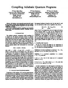
of state |ji (j = 1, 2, 3) is plotted in Fig. 2. As shown in Fig. 2(a), P3 increases from 0

8

Populations

(a)

P1 P2 P3

t/T (b)

Populations

P1 P2 P3

t/T

Po pulations

(c)

P1 P2 P3

t/T FIG. 2: The population Pj state of |ji versus t/T : (a) ϕ(T ) = π, κ = 1/2; (b) ϕ(T ) = 2π, κ = 1/4; (c) ϕ(T ) = 3π, κ = 1/6.

to 1 during the evolution, so the quantum transfer |1i → |3i can be achieved successfully. This proves that the method of the scheme and the replacing pulses in Eq. (15) are both effective. Fig. 2(a) also shows that P2 , the population of the intermediate state |2i, reaches

its maximal value P2max = 2κ − κ2 = 0.75 at t = T /2. If we want to decrease P2 , we can increase |ϕ(T )|, so that a smaller κ can be chosen. For example, if we choose ϕ(T ) = 2π, then κ = 1/4 can be adopted, so the maximal value of P2 is P2max = 2κ − κ2 = 0.4375 (See

9 Fig. 2(b)); if we choose ϕ(T ) = 3π, then κ = 1/6 is available, so the maximal value of P2 is P2max = 2κ − κ2 = 0.3056 (See Fig. 2(c)). However, increasing |ϕ(T )| requires us to increase e 0 should the maximal value of |ϕ|, ˙ since max |ϕ(t)| ˙ ≥ |ϕ(T )|/T (See Table I). As a result, Ω 0≤t≤T

e 0 × T (of the pulse also be increased. To have a relative high evolution speed, the product Ω e 0 and the total interaction time T ) is the smaller the better. Because when Ω e0 amplitude Ω

e 0 reaches the upper limit of the system), a smaller product Ω e 0 × T means a is fixed (e.g. Ω short interaction time T . On the other hand, in some cases, P2 is required to be restrained

in order to decrease the dissipation. Therefore, in real systems, one should choose a suitable value of control parameters for higher evolution speed and less dissipation. e 0 and the maximal value of intermediate state’s Table I. The pulse amplitude Ω population P2max with corresponding |ϕ(T )|.

P2max

π

e0 Ω

3.5/T

0.75

2π

6.2/T

0.4375

3π

8.0/T

0.3056

4π

9.5/T

0.2344

5π

10.7/T

0.1900

6π

11.8/T

0.1597

7π

12.8/T

0.1378

|ϕ(T )|

Now, we would like to show that the quantum transfer can be significantly accelerated by using the present scheme. As a comparison, the stimulated Raman adiabatic passage (STIRAP) is also exploited to implement the quantum transfer. According to STIRAP method, the system evolves through the dark state |Ψdark (t)i = √

1 (Ω2 (t)|1i Ω21 (t)+Ω22 (t)

−

Ω1 (t)|3i) of Hamiltonian H0 (t) shown in Eq. (1). By setting boundary condition lim =

t→−∞

Ω2 (t) Ω1 (t) = 0, lim = = 0, t→+∞ Ω2 (t) Ω1 (t)

(17)

one can design the Rabi frequencies Ω1 and Ω2 as following Ω1 (t) = Ω0 exp[−(

t − t0 − T /2 2 ) ], tc

Ω2 (t) = Ω0 exp[−(

t + t0 − T /2 2 ) ], tc

(18)

10

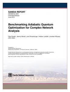
1-P 3 (T)

(units of 1/T) FIG. 3: 1 − P3 (T ) versus Ω0 for the STIRAP method.

where Ω0 denotes the pulse amplitude for STIRAP, t0 and tc are two related parameters. Setting t0 = 0.15T and tc = 0.2T , Rabi frequencies Ω1 and Ω2 can well satisfy the boundary condition in Eq. (17). We plot 1 − P3 (T ) versus Ω0 for the STIRAP method in Fig. 3. As shown in Fig. 3, with STIRAP, for obtaining an enough high population of state |3i, one should have Ω0 ≥ 45/T . When Ω0 = 70/T , 1 − P3 (T ) is 0.0002. For the present scheme, e 0 = 3.5/T . But for STIRAP, when Ω0 = 3.5/T , we have 1 − P3 (T ) ≤ 3.714 × 10−5 with Ω 1 − P3 (T ) = 0.9906 due to the great violation of the adiabatic condition. As we mentioned

above in this section, for a relatively high evolution speed, the product of the pulse amplitude and the total interaction time is the smaller the better. Therefore, using the present scheme, the quantum transfer can be significantly accelerated. At the end of this section, let us check the robustness of the scheme with some numerical simulations. Firstly, we would like to show the robustness of the scheme against the e1 parameters’ errors caused by the imperfect operations. Here, we consider the errors δT , δ Ω

e 2 of the total interaction time T , the Rabi frequencies of pulses Ω e 1 and Ω e 2 , respecand δ Ω

tively. Before we perform the numerical simulations, we assume that T ′ = T + δT is the e 1 /Ω e 1 and δ Ω e 2 /Ω e 2 are shown by the blue erroneous total interaction time. P3 (T ′ ) versus δ Ω

crosses and the solid-red line in Fig. 4, respectively. And P3 (T ′ ) versus δT /T is plotted by

the dashed-green line in Fig. 4. Seen from the dashed-green line in Fig. 4, we find that

11 P3 ( T ' )

relative errors e 1 /Ω e 1 (blue crosses), δΩ e 2 /Ω e 2 (solid-red line) and δT /T FIG. 4: P3 (T ′ ) versus relative errors: δΩ

(dashed-green line).

the scheme is quite robust against the timing errors, i.e., when |δT /T | ≤ 10%, we have

P3 (T ′ ) ≥ 0.9956. Besides, according to the blue crosses and the solid-red line in Fig. 4, the influences of pulses’ errors are larger than the timing error, however, P3 (T ) keeps higher

e 1 /Ω e 1 | ≤ 10% or |δ Ω e 2 /Ω e 2 | ≤ 10%. Therefore, the scheme holds nice than 0.9745 when |δ Ω

robustness against the parameters’ errors.

Secondly, let us analyze the robustness of the scheme against the decoherent factors. Here, we consider a superconducting (SC) qubit with Λ-type structure. For the SC qubit, there exists four decoherent factors: (i) the energy relaxation for the path |2i → |1i with energy relaxation rate Γ1 , (ii) the energy relaxation for the path |2i → |3i with energy relaxation rate Γ2 , (iii) the dephasing between energy levels |2i and |1i with dephasing rate Γφ1 , (iv) the dephasing between energy levels |2i and |3i with dephasing rate Γφ2 . Therefore, the evolution of the SC qubits can be described by a master equation in Lindblad form as following ρ˙ = i[ρ, H0 ] +

X l

1 [Ll ρL†l − (L†l Ll ρ + ρL†l Ll )], 2

(19)

where, Ll (l = 1, 2, 3, 4) is the Lindblad operator. Here, we have four Lindblad operators as L1 =

p

Γ1 |1ih2|,

L3 =

p

Γφ1 (|2ih2| − |1ih1|),

L2 =

p Γ2 |3ih2|, L4 =

p Γφ2 (|2ih2| − |3ih3|).

(20)

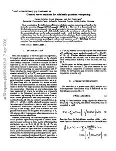
e 0 and Γ2 /Ω e 0 (Γφ1 /Ω e 0 and Γφ2 /Ω e 0 ) in Fig. 5 (a) (Fig. 5 (b)). Seen We plot P3 (T ) versus Γ1 /Ω

12 (a)

(b)

e 0 and Γ2 /Ω e 0 . (b)P3 (T ) versus Γφ1 /Ω e 0 and Γφ2 /Ω e 0. FIG. 5: (a)P3 (T ) versus Γ1 /Ω

e 0 ≤ 0.01 from Fig. 5 (a), P3 (T ) keeps higher than 0.986 for all Γ1 and Γ2 satisfying Γ1 /Ω e 0 ≤ 0.01. According to Fig. 5 (b), we have P3 (T ) ≥ 0.979 when Γφ1 /Ω e 0 ≤ 0.01 and Γ2 /Ω e 0 ≤ 0.01. Therefore, the scheme is also quite robust against energy relaxations and Γφ2 /Ω and dephasings for SC qubits. However, the SC qubits is more sensitive to dephasings when

using STIRAP, with pulses shown in Eq. (18), and parameters Ω0 = 45/T , t0 = 0.15T , tc = 0.20T , we have P3 (T ) = 0.9561 when Γφ1 /Ω0 = Γφ2 /Ω0 = 0.01. According to Refs. [8, 16], for a multi-qubit system which has an effective Hamiltonian in Λ-type structure, the dephasings influence the SQ very much when using STIRAP. For example, Ref. [16] has shown that with STIRAP, when the ratio between dephasing and coupling strength is only 0.0001, the fidelity of the target state falls from 1 to about 0.85. Therefore, the scheme may help to improve STIRAP for SC qubits.

III.

CONCLUSION

In conclusion, we have proposed an alternative scheme to construct a shortcut to the adiabatic passage via picture transformation for quantum transfer in a system with three-level Λ-type structure. Different from previous works [60–73], the present scheme has its own feature. For example, schemes [66–68] have adopted a serials of iterative picture transformations, while here picture transformation is used only once. Besides, the ideas of schemes [66–68] are to cancel the transitions between the eigenstates of iterative Hamiltonian in each

13 iterative picture, and the idea of scheme [73] suggests to cancel the transitions between a set of chosen dressed states. But for the present scheme, we directly study the dynamics of the three-level Λ-type system and the solution of the Schr¨odinger equation. Therefore, the present scheme consider the way to construct STAP from a different viewpoint. The present scheme has several advantages: (1) By choosing suitable control parameters, experimentally feasible pulses can be designed. (2) The quantum transfer can be achieved without any additional couplings. (3) Comparing with quantum transfer with adiabatic passages, the evolution is significantly sped up with present scheme. Since the three-level Λ-type structure is very common in all kinds of physical systems including superconducting qubits [7, 8, 16], quantum dots or NV centers [11, 68], boson gas in longitudinal coordinate coupled waveguides [1–4, 60, 74, 75], atoms trapped in the cavities [5, 6, 9, 10, 12–15], etc., the present scheme can be a choice to construct STAP in these physical systems. Considering the potential applications of the present scheme in experiments, we hope the present scheme may be useful in quantum information field.

ACKNOWLEDGEMENT

This work was supported by the National Natural Science Foundation of China under Grants No. 11575045, No. 11374054 and No. 11675046, and the Major State Basic Research Development Program of China under Grant No. 2012CB921601.

[1] M. Ornigotti, G. D. Valle, T. T. Fernandez, A. Coppa, V. Foglietti, P. Laporta, S. Longhi, J. Phys. B 41 (2008) 085402. [2] S. Longhi, Laser Photon. Rev. 3 (2009) 243-261. [3] S. Longhi, J. Phys. B 44 (2010) 051001. [4] A. A. Rangelov, N. V. Vitanov, Phys. Rev. A 85(2012) 055803. [5] Y. H. Chen, Y. Xia, Q. Q. Chen, J. Song, Phys. Rev. A 89 (2014) 033856. [6] M. Lu, Y. Xia, L. T. Shen, J. Song, N. B. An, Phys. Rev. A 89 (2014) 012326. [7] J. Zhang, T. H. Kyaw, D. M. Tong, E. Sj¨ovist, L. Kwek, Sci. Rep. 5 (2015) 18414. [8] X. Wei, M. F. Chen, Quantum Inf. Process. 14 (2015) 2419-2433.

14 [9] Y. H. Chen, Y. Xia, Q. Q. Chen, J. Song, Phys. Rev. A 91 (2015) 012325. [10] X. B. Huang, Z. R. Zhong, Y. H. Chen, Quantum Inf. Process. 14 (2015) 4475-4492. [11] X. K. Song, H. Zhang, Q. Ai, J. Qiu, F. G. Deng, New J. Phys. 18 (2016) 023001. [12] Y. H. Chen, Y. Xia, J. Song, Q. Q. Chen, Sci. Rep. 5 (2016) 15616. [13] Y. H. Chen, B. H. Huang, J. Song, Y. Xia, Opt. Comm. 380 (2016) 140-147. [14] Z. Chen, Y. H. Chen, Y. Xia, J. Song, B. H. Huang, Sci. Rep. 6 (2016) 22202. [15] W. J. Shan, Y. Xia, Y. H. Chen, J. Song, Quantum Inf. Process. 15 (2016) 2359-2376. [16] J. L. Wu, C. Song, J. Xu, L. Yu, X. Ji, S. Zhang, Quantum Inf. Process. 15 (2016) 3663-3675. [17] N. V. Golubev and A. I. Kuleff, Phys. Rev. A 90 (2014) 035401. [18] S. B. Zheng, Phys. Rev. Lett. 90 (2003) 217901. [19] S. B. Zheng, Phys. Rev. Lett. 95 (2005) 080502. [20] P. Kr´ al, I. Thanopulos, M. Shapiro, Rev. Mod. Phys. 79 (2007) 53-77. [21] K. Bergmann, H. Theuer, B. W. Shore, Rev. Mod. Phys. 70 (1998) 1003-1025. [22] M. P. Fewell, B. W. Shore, K. Bergmann, Aust. J. Phys. 50 (1997) 281-308. [23] N. V. Vitanov, T. Halfmann, B. W. Shore, K. Bergmann, Annu. Rev. Phys. Chem. 52 (2001) 763-809. [24] M. Demirplak, S. A. Rice, J. Phys. Chem. A 107 (2003) 9937-9945. [25] M. Demirplak, S. A. Rice, J. Chem. Phys. 129 (2008) 154111. [26] M. V. Berry, J. Phys. A 42 (2009) 365303. [27] E. Torrontegui, S. Ib´an ˜ez, S. Mart´ınez-Garaot, M. Modugno, A. del Campo, D. Gu´ery-Odelin, A. Ruschhaupt, X. Chen, J. G. Muga, Adv. Atom. Mol. Opt. Phys. 62 (2013) 117-169. [28] J. G. Muga, X. Chen, A. Ruschhaupt, D. Gu´ery-Odelin, J. Phys. B 42 (2009) 241001. [29] X. Chen, A. Ruschhaupt, S. Schmidt, A. del Campo, D. Gu´ery-Odelin, J. G. Muga, Phys. Rev. Lett. 104 (2010) 063002. [30] A. del Campo, M. G. Boshier, Sci. Rep. 2 (2012) 648. [31] X. Chen, I. Lizuain, A. Ruschhaupt, D. Gu´ery-Odelin, J. G. Muga, Phys. Rev. Lett. 105 123003 (2010). [32] A. del Campo, Phys. Rev. Lett. 111 (2013) 100502. [33] X. Chen, E. Torrontegui, J. G. Muga, Phys. Rev. A 83 (2011) 062116. [34] E. Torrontegui, S. Ib´an ˜ez, X. Chen, A. Ruschhaupt, D. Gu´ery-Odelin, J. G. Muga, Phys. Rev. A 83 (2011) 013415.

15 [35] J. G. Muga, X. Chen, S. Ib´an ˜ez, I. Lizuain, A. Ruschhaupt, J. Phys. B 43 (2010) 085509. [36] E. Torrontegui, X. Chen, M. Modugno, A. Ruschhaupt, D. Gu´ery-Odelin, J. G. Muga, Phys. Rev. A 85 (2012) 033605. [37] S. Masuda, K. Nakamura, Phys. Rev. A 84 (2011) 043434. [38] X. Chen, J. G. Muga, Phys. Rev. A 82 (2010) 053403. [39] J. F. Schaff, P. Capuzzi, G. Labeyrie, P. Vignolo, New J. Phys. 13 (2011) 113017. [40] X. Chen, E. Torrontegui, D. Stefanatos, J. S. Li, J. G. Muga, Phys. Rev. A 84 (2011) 043415. [41] E. Torrontegui, X. Chen, M. Modugno, S. Schmidt, A. Ruschhaupt, J. G. Muga, New J. Phys. 14 (2012) 013031. [42] A. del Campo, Eur. Phys. Lett. 96, 60005 (2011). [43] A. Ruschhaupt, X. Chen, D. Alonso, J. G. Muga, New J. Phys. 14 (2012) 093040. [44] J. F. Schaff, X. L. Song, P. Vignolo, G. Labeyrie, Phys. Rev. A 82 (2010) 033430. [45] J. F. Schaff, X. L. Song, P. Capuzzi, P. Vignolo, G. Labeyrie, Eur. Phys. Lett. 93 (2011) 23001. [46] X. Chen, J. G. Muga, Phys. Rev. A 86 (2012) 033405. [47] A. C. Santos, M. S. Sarandy, Sci. Rep. 5 (2015) 15775. [48] A. C. Santos, R. D. Silva, M. S. Sarandy, Phys. Rev. A 93 (2016) 012311. [49] I. Hen, Phys. Rev. A 91 (2015) 022309. [50] M. S. Sarandy, L. A. Wu, D. Lidar, Quantum Inf. Process. 3 (2004) 331-349. [51] I. B. Coulamy, A. C. Santos, I. Hen, M. S. Sarandy, Front. ICT 3 (2016) 19. [52] M. M. Rams, M. Mohseni, A. del Campo, New J. Phys. 18 (2016) 123034. [53] S. Deffner, C. Jarzynski, A. del Campo, Phys. Rev. X 4 (2014) 021013. [54] A. del Campo, Phys. Rev. A 84 (2011) 031606(R). [55] Y. X. Du, Z. T. Liang, Y. C. Li, X. X. Yue, Q. X. Lv, W. Huang, X. Chen, H. Yan, S. L. Zhu, Nat. Commun. 7 (2016) 12479. [56] S. An, D. Lv, A. del Campo, K. Kim, Nat. Commun. 7 (2016) 12999. [57] L. Giannelli, E. Arimondo, Phys. Rev. A 89 (2014) 033419. [58] S. Masuda, S. A. Rice, J. Phys. Chem. A 119 (2015) 3479. [59] M. G. Bason, M. Viteau, N. Malossi, P. Huillery, E. Arimondo, D. Ciampini, R. Fazio, V. Giovannetti, R. Mannella, O. Morsch, Nat. Phys. 8 (2012) 147. [60] S. Mart´ınez-Garaot, E. Torrontegui, X. Chen, J. G. Muga, Phys. Rev. A 89 (2014) 053408.

16 [61] T. Opatrn´ y, K. Mømer, New J. Phys. 16 (2014) 015025. [62] H. Saberi, T. Opatrn´ y, K. Mømer, A. del Campo, Phys. Rev. A 90 (2014) 060301(R). [63] E. Torrontegui, S. Mart´ınez-Garaot, J. G. Muga, Phys. Rev. A 89 (2014) 043408. [64] B. T. Torosov, G. D. Valle, S. Longhi, Phys. Rev. A 87 (2013) 052502. [65] B. T. Torosov, G. D. Valle, S. Longhi, Phys. Rev. A 89 (2014) 063412. [66] S. Ib´an ˜ez, X. Chen, E. Torrontegui, J. G. Muga, A. Ruschhaupt, Phys. Rev. Lett. 109 (2012) 100403. [67] S. Ib´an ˜ez, X. Chen, J. G. Muga, Phys. Rev. A 87 (2013) 043402. [68] X. K. Song, Q. Ai, J. Qiu, F. G. Deng, Phys. Rev. A 93 (2016) 052324. [69] B. H. Huang, Y. H. Chen, Q. C. Wu, J. Song, Y. Xia, Laser Phys. Lett. 13 (2016) 105202. [70] Y. H. Chen, Q. C. Wu, B. H. Huang, Y. Xia, J. Song, Phys. Rev. A 93 (2016) 052109. [71] Y. H. Chen, J. Song, Y. Xia, Sci. Rep. 6 (2016) 38484. [72] Y. H. Kang, Y. H. Chen, Q. C. Wu, B. H. Huang, Y. Xia, J. Song, Sci. Rep. 6 (2016) 30151. [73] A. Baksic, H. Ribeiro, A. A. Clerk, Phys. Rev. Lett. 116 (2016) 230503. [74] M. P. A. Fisher, P. B. Weichman, G. Grinstein, D. S. Fisher, Phys. Rev. B 40 (1989) 546-570. [75] D. Jaksch, C. Bruder, J. I. Cirac, C. W. Gardiner, P. Zoller, Phys. Rev. Lett. 81 (1998) 3108-3111.