Accelerating Collaborative Filtering Using Concepts from High ...

2015 IEEE International Conference on Big Data (Big Data)

Accelerating Collaborative Filtering Using Concepts from High Performance Computing Mark Gates, Hartwig Anzt, Jakub Kurzak, Jack Dongarra Innovative Computing Lab University of Tennessee Knoxville, USA {mgates3,hanzt,kurzak,dongarra}@icl.utk.edu Abstract—In this paper we accelerate the Alternating Least Squares (ALS) algorithm used for generating product recommendations on the basis of implicit feedback datasets. We approach the algorithm with concepts proven to be successful in High Performance Computing. This includes the formulation of the algorithm as a mix of cache-optimized algorithm-specific kernels and standard BLAS routines, acceleration via graphics processing units (GPUs), use of parallel batched kernels, and autotuning to identify performance winners. For benchmark datasets, the multi-threaded CPU implementation we propose achieves more than a 10 times speedup over the implementations available in the GraphLab and Spark MLlib software packages. For the GPU implementation, the parameters of an algorithm-specific kernel were optimized using a comprehensive autotuning sweep. This results in an additional 2 times speedup over our CPU implementation. Index Terms—Collaborative Filtering; Alternating Least Squares; GPUs; Autotuning; Batched Cholesky

collected. Explicit feedback systems collect customer ratings, such as star ratings or thumbs up/down as a numerical value. Implicit feedback systems exclusively monitor users’ behavior. This can be the purchase or browsing history, search patterns, or even mouse movements [4]. For this type of collaborative filtering, Hu et al. recently proposed [4] a new algorithm that allows for the efficient recommendation generation with a high matching accuracy, reviewed in Section II. As we are convinced of its high significance, we propose in this paper multi-core CPU and GPU implementations for the suggested algorithm that are able to exploit the computing power of state-of-the-art processors and accelerators. We compare performance with the open source implementations available in Mahout [8], GraphLab [9], and Spark MLlib [10], [11], and report significant speedups for selected benchmark datasets. II. C OLLABORATIVE F ILTERING

I. I NTRODUCTION The growing popularity of web-based services such as movie databases and online retailers raises the problem of how customers can easily find products fitting their preferences. As addressing this challenge is one of the key factors determining the success of an online service, significant effort has been spent on developing recommendation systems [1], [2], [3], [4] that provide personalized product suggestions to a specific user. There exist several strategies of how these recommendations are generated. Content-based recommendation systems require a profile for each user and each product containing information like age, gender, and nationality of users; and genre, size, and color of items. Matching algorithms then associate customers with products. Though typically very accurate, an obvious drawback of this recommendation strategy is that collecting data requires explicitly populating the database with profiles. For this reason, much attention has been drawn to content-free recommendation systems that rely on only past user behavior, without requiring the creation of user or product profiles [4]. Content-free recommendation systems based on the Collaborative Filtering (CF) approach [2], [5] harvest information collected by a large number of former users to suggest certain products to a specific customer. Typical applications are web-based music or movie services like Yahoo [6] or Netflix [7]. Content-free recommendation systems can be categorized into two subgroups that differ in the way the data is 978-1-4799-9926-2/15/$31.00 ©2015 IEEE

CF algorithms are based on observation data stored in a relation matrix, R. For explicit feedback, the value rui indicates how a user u rated item i. For implicit feedback, the value rui represents the observation value for this useritem combination. This can be the number of website visits, amount of time spent watching this item, or the number of times the customer purchased this product. An obvious result of these strategies is that most rui entries are zero. However, only the non-zero values provide useful information, as a value may be zero for very different reasons: the user may dislike a product, or may just not be aware of it. To account for the low confidence in the missing data, Hu et al. propose [4] the use of binary values,  1 if rui > 0, pui = 0 if rui = 0, to indicate whether a user u has a preference for item i. But also the observations rui may carry some noise, as a user may stay on a webpage because he left the computer, or purchase an item for a friend—despite not liking it for himself. In general, however, larger values of rui indicate stronger preference. A workaround to account for this uncertainty in the values rui > 0 is to introduce a matrix C with entries cui that measure the confidence of the observation pui via cui = 1 + αrui . 667

function ALS( input: α, λ, R; output: X, Y ) set Y to random initial guess while not converged // update user-factors X for u = 1, . . . , m  solve Y C u Y T + λI xu = Y C u pu for xu end // update item-factors Y for i = 1,. . . , n  solve XC i X T + λI yi = XC i pi for yi end check for convergence end end function

With increasing α reflecting more confidence, experiments have revealed α = 40 provides good results [4]. The algorithm now tries to find a vector xu for each user u and a vector yi for each product i that reflects the user preferences. These vectors xu and yi are of length f , representing the feature space size. In some sense, f represents the number of categories into which users and items will be grouped. However, these categories are implicit, without any explicit, a priori meaning assigned to each category. The feature space size f is typically small compared to the number of users and items, e.g., from 10 to 100, depending on the application. The user-factors xu and item-factors yi are computed such that their inner product approximates in a least-squares sense the preference pui correlating user u to item i, xTu yi ≈ pui .

Fig. 1. Pseudocode of alternating least square algorithm iterating user-factors and item-factors.

The factors xu and yi can be computed by minimizing the cost function       2 2 2 T min cui pui − xu yi + λ xu  + yi  . u,i

u

R m users

x∗ ,y∗

n items

i

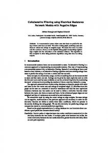
(1) For m users and n products, the above sum contains mn terms, which can for a real-world application quickly exceed a few billion [4]. This huge number prohibits the efficient use of techniques like stochastic gradient descent, which motivated Hu et al. to derive a different optimization technique based on the observation that if either the user-factors or the itemfactors are fixed, the cost function becomes quadratic, so an alternating least square (ALS) algorithm can be used to solve the problem, as outlined in Figure 1. In the first step, the userfactors are updated for fixed item-factors. For this purpose, let Y be a wide f × n matrix of all item-factors, with each yi being one column. Furthermore, for each u, let C u be an n × n diagonal matrix, with diagonal entries from row u of C, such that cuii = cui , as depicted in Figure 2. Let pu be a vector containing all the preferences of u (the pui values). Differentiating the cost function (1) allows us to express the minimum for the user-factor as  −1 xu = Y C u Y T + λI Y C u pu . (2) This step is repeated for all users, i.e., m times. The resulting user-factors are gathered in a wide f × m matrix X, with each xu being one column. In the next step, the item-factors are updated in a similar fashion: using the diagonal m × m matrix C i , with diagonal entries from column i of C, such that ciuu = cui , and the vector pi , the minimum item-factor for fixed user-factors is given as  −1 yi = XC i X T + λI XC i pi . (3) This step is repeated for all items, i.e., n times. After this computation, the updated item-factors are gathered in the f × n matrix Y , and the user-factors can be updated again.

u

Au

Y = f×n f×f for users u = 1, ..., m

R n×n

T

Y n×f

+ YYT + λ I

Ri m×m Ai f×f

X f×m

=

XT m×f

T

+ XX + λ I

for items i = 1, ..., n Fig. 2. Diagram of computation of user-factors and item-factors. R is general sparse, Ru and Ri are sparse diagonal, X, Y, Au , Ai are dense.

Alternating between these two steps minimizes the cost function. Experiments have shown that the user- and item-factors typically converge after a few iterations [4]. The two steps, updating the user-factors and the itemfactors, are identical except for swapping the input and output matrices. Therefore, in the remainder of the paper we will focus on updating the user-factors, and the item-factors will follow similarly. For computational efficiency, the product can be factored as Y C u Y T = Y Y T + αY Ru Y T , u = rui where Ru is a sparse diagonal matrix with entries rii from row u of R. As Y Y T is the same for all users, it can be computed once per iteration [4]. This yields a dense rank-k update for Y Y T , which is efficiently implemented in the syrk

668

function ALS( input: R; output: X, Y ) set Y to random initial guess while not converged // update user-factors X set BLAS to multi threaded Z = Y Y T using syrk BLAS set BLAS to single threaded parallel for u = 1, ..., m ALS CORE ( ru,: , Y, Z, xu ) to solve (Y C u Y T + λI)xu = Y C u pu end // update item-factors Y set BLAS to multi threaded Z = XX T using syrk BLAS set BLAS to single threaded parallel for i = 1, ..., n ALS CORE ( r:,i , X, Z, yi ) to solve (XC i X T + λI)yi = XC i pi end check for convergence end end function

T

Y W

Y

A

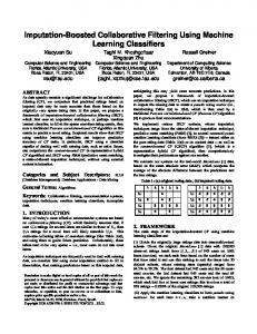
ru Fig. 3. Schematic of A = Y Ru Y T . Dark boxes represent non-zeros in row ru . Only corresponding columns of Y and rows of Y T contribute to A.

(symmetric rank-k update) BLAS routine. The remaining term, αY Ru Y T , involves a dense matrix Y and the sparse diagonal matrix Ru , which will require a custom kernel to implement. With the very mild assumption that Y is full rank, i.e., has f linearly independent rows, the product Y Y T is symmetric positive definite (SPD). Assuming Ru contains only nonnegative implicit feedback data like webpage hits or ratings, and α, λ ≥ 0, the entire term Y Y T + αY Ru Y T + λI will be SPD, allowing us to solve it with the Cholesky factorization. III. CPU

Fig. 4. Multi-core CPU ALS algorithm.

function ALS CORE( input: ru,: , Y, Z; output: x ) // A, b are local workspaces A=0 b=0 for k = column indices of non-zeros in row ru,: A += ruk yk ykT b += (1 + αruk )yk end A = Z + αA + λI solve Ax = b for x using Cholesky end function

IMPLEMENTATION

In the product Y Ru Y T , the sparse diagonal matrix Ru can be seen as selecting a few columns of Y , plus scaling columns, as shown in Figure 3. Columns of Y corresponding to zeros in Ru can be ignored. As k, the number of non-zeros in Ru , is typically much less than n, the number of columns of Y (see Figure 12), the kernel should take advantage of this sparsity. This reduces the cost from a rank-n update to a rank-k update, with k  n. For instance, with the Million Song dataset, described in Section VI, and f = 64, the problem is to generate and solve m = 1019318 systems, each formed by a 64 × 64 rank-k update, with the average k = 126. There is not enough parallelism in a single system for an efficient multicore implementation. Instead, we do a batched implementation that generates and solves the m systems in parallel. For this, we use OpenMP to parallelize the loops in Figure 4. The ALS CORE routine solves each user-factor xu and item-factor yi , and runs single-threaded within each OpenMP thread. A simple, Level 2 BLAS implementation of ALS CORE is shown in Figure 5. This loops over the non-zeros in each row u of R, accumulating outer products, A += ruk yk ykT . The right-hand side b is also computed at the same time, to optimize cache reuse of yk . Each outer product does O(n2 ) work on O(n2 ) data, leading to a memory-bound algorithm. Better efficiency can be attained by relying on optimized Level 3 BLAS routines, as shown in Figure 6. Level 3 BLAS routines operate on matrices instead of individual vectors,

Fig. 5. CPU kernel to update one user-factor x, Level 2 BLAS implementation.

function ALS CORE( input: ru,: , Y, Z; output: x ) // A, b, V, W are local workspaces b=0 j=1 for k = column indices of non-zeros in row ru,: // copy relevant columns of Y to V and W vj = ruk yk wj = yk b += (1 + αruk )yk j += 1 end A = Z + αV W T + λI using gemm or syrk BLAS solve Ax = b for x using Cholesky end function Fig. 6. CPU kernel to update one user-factor x, Level 3 BLAS implementation.

669

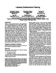
enabling data reuse and optimizations for cache efficiency, improving performance to be compute-bound instead of memorybound. To use Level 3 BLAS, we copy the relevant columns of Y to workspaces V and W , with the column scaling included in V , then use a gemm (general matrix-matrix multiply) BLAS call. If all non-zero entries of R are 1, as might be the case for a thumbs-up/down rating, then V = W , so instead of gemm we can use a syrk BLAS call, which computes only the lower triangle of the symmetric matrix A, reducing work by half. Updating the item-factors is exactly the same, except it uses columns of R instead of rows of R. For updating the userfactors, we store R in CSR (compressed sparse row) format, which gives efficient, contiguous access to each row of R, but slow access to columns of R. For efficiency in updating the item-factors, we also store R in CSC (compressed sparse column) format, which gives efficient, contiguous access to each column of R. Because the number of non-zeros per row can vary significantly (see Figure 12), there will be a load imbalance between different processors. This is easily solved by using the OpenMP dynamic scheduler, adding schedule(dynamic,NB), with a block size NB. We set NB = 200, but performance is not sensitive to the exact value. IV. GPU A RCHITECTURE Before describing our GPU implementation in Section V, we will briefly review relevant aspects of the GPU architecture that dictate algorithmic choices. The two most prominent features of GPUs are the Single Instruction Multiple Thread (SIMT) architecture and the memory model. A GPU computation is divided into a 1D, 2D, or 3D grid of thread blocks. Thread blocks execute independently; there is not an easy method to synchronize or exchange data between thread blocks. A thread block is further organized as a 1D, 2D, or 3D grid of threads. These threads are not independent, but in SIMT fashion must follow the same execution path in lock-step, possibly with some threads disabled to handle conditionals. Within a thread block, threads can synchronize and exchange data via shared memory. Specific hardware features (e.g., warps and coalesced reads) affect performance and so determine optimal configurations of thread blocks. Figure 7 shows the hardware architecture of NVIDIA GPUs. The basic execution unit is a CUDA core, which executes a single floating point operation per cycle. Cores are organized into multiprocessors. Each thread block is assigned to a multiprocessor, and each multiprocessor can execute multiple thread blocks. A thread block is executed in sets of 32 threads, called a warp. In the Kepler architecture, a multiprocessor contains 192 cores, and the GPU contains up to 15 multiprocessors, for a total of 2880 cores. The Kepler multiprocessor also contains a large register file of 65,536 32-bit registers, and 64 KB of fast memory that serves as L1 cache and shared memory. Shared memory is a type of memory specific to GPUs, introduced to allow for exchanging data among cores. Conceptually, it is more an extension of the register file than a cache. A thread block statically allocates arrays in shared

Fig. 7. Architecture of NVIDIA GPUs.

memory, which are then accessible by all threads in the thread block. The fastest memory in the multiprocessor is the register file. Registers are partitioned among threads and each thread has a private set of registers. The second fastest memory is the shared memory and L1 cache. The slowest memory in the system is main GPU memory in DRAM. Reads from DRAM pass through the L2 cache and either the L1 cache or read-only data cache. DRAM bandwidth is a precious commodity for batched matrix operations, which are very close to being memory bound. V. GPU

IMPLEMENTATION

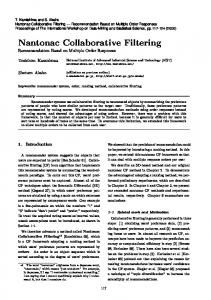
Due to the GPU architecture, the GPU implementation, shown in Figure 8, is structured differently than the CPU implementation in Figure 4. Multiple thread blocks work to compute each matrix Au , after which each matrix can be solved. As with the CPU implementation, a single system has insufficient parallelism to fill the GPU. Therefore, to fully occupy all of the GPU’s cores, we use a batched implementation, where a single GPU kernel generates a batch of Au matrices using the BATCHED SPARSE SYRK routine, then a batched Cholesky routine factors them, and finally batched triangular solvers solve the resulting systems. We use the batched Cholesky and triangular solves from the BEAST open source package [12]. The implementation of the BATCHED SPARSE SYRK GPU kernel is given in Figure 9 and shown schematically in Figure 10. A 3D grid of thread blocks is used. One dimension covers the batch of s systems to be formed, A1 , . . . , As . The memory requirement is O(f m + f n + sf 2 + z), where z is the number of non-zeros in R. To minimize the memory used, we use a modest batch size of s = 4096 systems, rather than launching a single batch of s = m systems. The other two grid dimensions divide each Au matrix into an n/nb × n/nb grid of tiles of size nb × nb (light orange in Figure 10). Each tile will be handled by one thread block on the GPU. 670

function ALS GPU( input: R; output: X, Y ) // workspaces: A is f × f × s, B is f × s set Y to random initial guess while not converged // update user-factors X Z =YYT for u = 1, . . . , m by batch size s BATCHED SPARSE SYRK ( u, R, Y, Z, A, B ) to compute Aj = (Y C j Y T + λI) and bj = C j Y pj for j = u, . . . , u + s BATCHED CHOLESKY ( A ) to factor Aj for j = u, . . . , u + s BATCHED SOLVE ( A, B, xu:u+s ) to solve Aj xj = bj for j = u, . . . , u + s end // update item-factors Y Z = XX T for i = 1, . . . , n by batch size s BATCHED SPARSE SYRK ( i, R, X, Z, A, B ) to compute Aj = (XC j X T + λI) and bj = C j Xpj for j = i, . . . , i + s BATCHED CHOLESKY ( A ) to factor Aj for j = i, . . . , i + s BATCHED SOLVE ( A, B, yi:i+s ) to solve Aj yj = bj for j = i, . . . , i + s end check for convergence end end function

function BATCHED SPARSE SYRK( input: u, R, Y ; output: A, B ) // has f /nb × f /nb × (batch size s) thread blocks // rA is (nb/dx) × (nb/dy) registers per thread // sY is nb × kb elements, shared // sY T is nb × kb elements, shared // sR is kb elements, shared (bx, by, bz) = thread block indices rA = 0 j = u + bz for p = R.rowptr[j], . . . , R.rowptr[j + 1] by step kb load sR = R.values[p : p + kb] load cols = R.colind[p : p + kb] load sY = Y [bx ∗ nb : (bx + 1) ∗ nb, cols] load sY T = Y [by ∗ nb : (by + 1) ∗ nb, cols] synchronize threads for k = 0, . . . , kb − 1 rA[0 : nb, 0 : nb] += sR[k]∗sY [:, k]∗sY T [:, k]T end synchronize threads end save rA to (bx, by) tile of Aj end function Fig. 9. Batched sparse-syrk GPU kernel. Operations have implicit inner loops for sub-tiling the given ranges by dx × dy threads, which are omitted for simplicity.

Fig. 8. GPU implementation of ALS, using batched operations.

{

nb

Each tile is further subdivided into sub-tiles of size dx × dy (dark orange), corresponding to the thread dimensions of the thread block, i.e., each thread block has dx × dy threads. We require that dx and dy both evenly divide nb. Each thread is responsible for (nb/dx)×(nb/dy) entries in the output matrix A. In Figure 10, each thread computes 6 entries, one in each sub-tile of rA. Intermediate values are stored in registers in rA; at the end, the final sum is saved back to main GPU memory in A. The algorithm proceeds by loading kb non-zero values of ru and their column indices. For off-diagonal blocks, an nb × kb portion of Y is loaded into shared memory in sY (blue in Figure 10) from the kb columns corresponding to non-zero values in ru . Likewise, a kb × nb portion of Y T is loaded into shared memory in sY T (red). The shared memory matrices sY and sY T are also sub-tiled by the dx × dy thread block, and we further required that dy evenly divides kb. After loading, all the threads synchronize to ensure that data loads have completed. Then each thread loops over the kb columns in sY and sY T , performing a rank-1 outer-product update of rA for each pair of columns. This is repeated, loading the next kb non-zero values of ru , until the entire row has been processed. Finally, the results are saved from rA in registers

YT

{

nb

kb

rA

nb

{

{

{

sR

sYT

dx

{

sY dy

Y

A

{

nb

ru Fig. 10. Schematic of sparse-syrk GPU kernel.

671

Dataset rec-eachmovie Million Song Dataset Netflix Challenge Yahoo! Song Dataset

# users 1,623 1,019,318 480,190 130,558 TABLE I

# items 61,265 384,546 17,771 136,736

# edges 2,811,717 48,373,586 100,480,508 49,770,695

0

500

DATASET PROPERTIES 1000

to A in main GPU memory. For diagonal blocks, a similar procedure is followed, with two changes. The portion that would be loaded into sY T is identical to sY , so loading sY T can be skipped. Also, only the lower triangle needs to be saved, as shown in gray in Figure 10. The upper triangle is known implicitly by symmetry. The diagonal blocks also accumulate the right hand side, bj . A few optimizations can be made. Only the tiles on or below the diagonal need to be computed; tiles above the diagonal are known by symmetry. Also, since matrix Y is read-only, it is beneficial to bind its memory to GPU texture memory, which has optimized caching for read-only data. Texture memory also simplifies the code by dealing with outof-bounds memory accesses in hardware—the software can pretend that Y is bigger than it actually is. This allows for fixed loop bounds and eliminates cleanup code, enabling more compiler optimizations. When saving data from rA to A at the end, bounds are checked so no invalid data is written back to memory. VI. I MPLICIT F EEDBACK DATASETS We use different recommendation datasets to ensure correct convergence and to compare the performance of the developed CPU and GPU implementation to the reference implementations that are part of popular software packages used for data analytics. In the runtime comparisons, we target the Million Song Dataset [13], the Netflix Challenge Dataset [14], [7], and the Yahoo! Song Dataset [6]. To identify a good parameter configuration for the GPU implementation, we employ an autotuning sweep using the BEAST framework [15]. For this purpose, we choose rec-eachmovie, a significantly smaller dataset that allows for executing a comprehensive set of kernel configurations in a moderate runtime. Like the Netflix Challenge, it contains data connecting users to movies [16]. All datasets are listed along with some key properties in Table I. For the Million Song Dataset, we visualize in Figure 11 the nonzero pattern of the first 2000 rows of the adjacency matrix. Although this is only a small portion of the data, it already allows us to identify some typical characteristics in the sparsity pattern: • For all users u and items i with i > u, ru,i = 0. • There exist some users who have listened to a lot songs (many entries in one row) and others who have listened to only few (few entries in a row). This results in a structure of horizontal lines. Furthermore, for users who have listened to many songs, there is a high chance that

1500

2000 0

10000

20000

30000

40000

Fig. 11. Sparsity structure of subset of Million Song Dataset.

they have also listened to songs that none of the previous users have listened to before. • There exist popular songs (many entries in a column) and unpopular songs (few entries in a column). This gives the vertical stripes in the sparsity plot. • For a popular song, chances are low that a user with a high ID is the first who has listened to it. Therefore, there is a tendency for the columns to become less dense when going from left to right. For all target databases, we visualize in Figure 12 the nonzero distribution. Each bar of the histograms represents the number of rows (left-hand plot) or columns (right-hand plot) with a certain number of nonzeros. The minimum, median, mean, and maximum number of nonzeros per row and column are annotated in each graph. As previously noted, the wide range of nonzeros per row and column means different users and items incur widely different costs in computing Y C u Y T and XC i X T , potentially leading to load imbalance. VII. H ARDWARE AND S OFTWARE S ETUP For comparison, we chose three ALS implementations from data analytics software stacks: Mahout (version 0.9) [8], [17] GraphLab (version 1.3) [9], [18], [19], and Spark MLlib (version 1.5) [20]. All these software packages support multithreading and are popular in data analytics. The runtime results for our developed CPU implementation, Mahout, GraphLab, and Spark MLlib were obtained on a twosocket Intel Sandy Bridge Xeon E5-2670 running at 2.6 GHz, featuring 8 cores in each socket, with a theoretical peak of 666 Gflop/s in single precision and 333 Gflop/s in double precision. The system has 64 GB of main memory that can be accessed at a theoretical bandwidth of 51 GB/s. All CPU implementations were linked against Intel’s Math Kernel Library (MKL) version 11.1.2 [21]. GPU results are on an NVIDIA Kepler K40c with 15 multiprocessors, each containing 192 CUDA cores. The theoretical peak floating point performance is 4,290 Gflop/s in single precision and 1,682 Gflop/s in double precision. On the GPU, 12 GB of main memory can be accessed at a 672

Million Song

Netflix

Yahoo! Song

Fig. 12. Nonzero distribution of rows (top) and columns (bottom) of target datasets.

theoretical bandwidth of 288 GB/s. The implementation of all GPU kernels is realized in CUDA version 7.0 [22]. VIII. AUTO T UNING The optimal parameters for the sparse-syrk GPU kernel are not obvious and not easy to derive by an analytical formula. Therefore the factorization calls for a real autotuning sweep. To achieve high performance, classic heuristic automatic software tuning methodology is applied, where a large number of kernels are generated and run, and the fastest ones identified. Different values are possible for the tile size nb, block size kb, and thread block dimensions dx and dy. The kernel is generalized so that any value of nb can be used for any feature space size f . The BEAST autotuning framework enumerates and tests all possible kernel configurations. Various constraints are applied to limit the search space. Correctness constraints include that nb is divisible by dx and dy, and that kb is divisible by dy. These ensure that sub-tiles exactly cover the matrix tile. Additional constraints include hardware limits: maximum threads per thread block, maximum registers per thread, maximum registers per thread block, and maximum shared memory per thread block. Configurations violating those constraints would either not compile or not run correctly. To further eliminate kernels that are unlikely to perform well, we also applied several soft constraints. These include: thread block size is a multiple of the warp size, ratio of load instructions to multiply-add instructions is not below a threshold (0.5), and the number of threads that can be scheduled on each multiprocessor (occupancy) is not below a threshold (512). While kernels that violate these soft constraints will run correctly, they will not keep the GPU fully occupied, leading to lower performance. After applying these constraints, BEAST generated 330 kernel configurations to test. The kernels were tested on the

modest sized rec-eachmovie dataset, timing the sparse-syrk for both the user-factor and the item-factor matrix generation. Due to differences in the size of Y and X and the sparsity of Ru and Ri , the performance was not identical between these two. We ran tests for sizes of f that are multiples of 8 and multiples of 10, from 8 to 100. The performance of all these kernels is plotted in gray in Figure 13. Kernels that were best for some size are highlighted with colored markers. For each size f , the circled kernel was chosen as the best overall kernel, having the highest geometric mean performance between the user-factor and the item-factor performance. Configurations are specified by a tuple (nb, kb, dx, dy). Inspecting the data reveals that no one kernel was optimal across all feature space sizes. Taking the yellow diamond (80, 8, 16, 16) kernel as an example: for small f it is a poor performer, but the performance increases as f increases, until it is the best kernel for f = 80, where f = nb. For the next size, f = 88, its performance plummets to less than half the optimal performance. This occurs because it goes from one tile to four tiles covering each matrix A, wasting three large tiles to cover the extra 8 rows and columns. This saw tooth pattern is evident for all the configurations. While often the best kernel for user-factors (left in Figure 13) and item-factors (right) is the same, there are several instances where this is not true. At f = 48, the blue diamond (48, 8, 16, 16) is best for user-factors, but the red diamond (48, 8, 8, 16) is best for item-factors. The red diamond is chosen as best overall, but loses 12% of the optimal performance for user-factors. In a couple instances, the best overall kernel is not the best for either user-factors or item-factors, but the best compromise between the two. At k = 32, the green circle (32, 8, 16, 16) is chosen instead of the top performers, the yellow circle (32, 8, 32, 16) and red circle (32, 8, 8, 8). While the performance does depend on the sparsity pattern— 673

Y CuY T

450 400

250

350

200

250

Gflop/s

Gflop/s

300

200 150

150 100

100

50

50 0

XC i X T

300

10

20

30

40

50

60

70

80

90 100

0

10

20

feature space size f

30

40

50

60

70

80

90 100

nb, kb, dx, dy 16, 8, 8, 8 16, 4, 20, 8 24, 4, 8, 8 24, 8, 8, 8 24, 8, 24, 8 32, 8, 8, 8 32, 8, 8, 16 32, 8, 16, 16 32, 8, 32, 16 40, 8, 8, 8 48, 8, 8, 16 48, 8, 16, 16 64, 8, 8, 16 80, 8, 16, 16

feature space size f

Fig. 13. Performance of all kernels (gray lines), highlighting ones that are best for some size. Circled kernel is chosen as best for each size.

and therefore on the dataset—none of the chosen kernels performed poorly in either case, losing at most 22% of the optimal performance. This analysis highlights the need for autotuning. The performance difference between the best and worst kernels is dramatic—between a factor of 6 and 72 times for a particular f . Also, the optimal kernel configuration depends heavily on the size f , and to a lesser extent on the actual dataset. While some kernel configurations make sense in retrospect, such as nb = 80 for f = 80, it was infeasible to predict optimal kernels in all cases. IX. P ERFORMANCE E VALUATION We first ran performance scaling studies of the ALS algorithm in the Mahout, GraphLab, and Spark reference implementations to ensure correct usage. Figure 14 shows time vs. number of cores for the rec-eachmovie dataset with feature space size f = 96 in log-log scale. Perfect linear scaling would be a straight line, as shown by the dashed lines. This was a small enough dataset that running a complete parallel scaling study was feasible; however, due to its small size, we would not expect linear scaling. Mahout scales well, achieving slightly super-linear parallel speedup (usually due to a larger combined cache on multiple cores), with 18.3 times parallel speedup on 16 cores over its single core performance. GraphLab scales reasonably well for this small problem, achieving 9.6 times parallel speedup on 16 cores. Spark exhibited worse scaling, with a 6.9 times parallel speedup on 16 cores. Our own CPU implementation scales nearly linearly up to 4 cores, then loses some parallel efficiency for more cores, achieving 8.3 times speedup on 16 cores. For the larger datasets shown in Figure 15, it achieves better efficiency, up to 14.1 times parallel speedup for the Netflix dataset. Similar parallel speedups are achieved for different feature space sizes, ranging from 11.5 to 14.6 times on 16 cores.

Fig. 14. Parallel scaling in log-log scale for rec-eachmovie dataset with f = 96.

Fig. 15. Parallel speedup of CPU implementation for f = 64.

674

Fig. 16. Time in log scale (left) and linear scale (right) for single ALS iteration, using 16 cores.

The large performance difference between implementations is evident in the parallel scaling. Mahout is nearly two ordersof-magnitude slower than GraphLab and Spark. This is not surprising, as Mahout is written in Java while GraphLab is a newer implementation written in C++. Spark, while written in Scala/Java, links with native optimized BLAS to achieve good performance. GraphLab is an order-of-magnitude slower than our CPU implementation, while for this small problem size, Spark is 2 to 3 times faster than GraphLab, and 4 to 5 times slower than our CPU implementation. For the three large benchmark databases—Netflix, Million Song, and Yahoo! Song—execution time for a single ALS iteration (updating user-factors and item-factors once) is presented in Figure 16, in both log and linear scale. This covers a range of feature space sizes, all using 16 cores or the GPU. As it was clear that Mahout was a slow performer, we did not do a complete sweep of its sizes. With these larger datasets, Spark is slower than GraphLab for small f . For larger f ≥ 50 with the Yahoo! Song and Netflix datasets, Spark had performance comparable to GraphLab. However, with the Million Song dataset, the Spark execution time increased markedly for f ≥ 50, and it encountered an exception for f ≥ 80. Examining our GPU performance in detail, there are a few notable plateaus that occur from f = 10 to 16, from f = 40 to 48, and from f = 50 to 64. All these ranges end at multiples of 16, which are sizes that often do well on GPU hardware due to matching the size of warps and coalesced reads (a kind of vector load). Nonetheless, performance remains good across a variety of sizes. The speedup of our GPU implementation over Mahout, GraphLab, Spark, and our CPU implementation is given in Figure 17. The GPU achieves between 1.2 and 2.9 times speedup, with average 2.1 times, over our CPU implementation. Compared to GraphLab, the GPU achieves from 11.5 to 29.9 times speedup, with an average of 20.9. Compared to

Fig. 17. Speedup in log scale of GPU implementation over Mahout, GraphLab, Spark, and CPU implementations using 16 cores.

Spark, it achieves from 12.6 to 74.9 times speedup, with an average of 35.3. Mahout performs poorly, taking 1684 times longer, on average, to compute a single ALS iteration. While speedups are similar across datasets, our GPU implementation consistently gets the best speedups for the Netflix dataset and the least speedups for the Million Song dataset. This may be because the Million Song dataset has the smallest average nonzeros-per-row and nonzeros-per-column, with a mean of 47 nonzeros per row and 126 per column, compared to 209 and 5654 for the Netflix dataset (Figure 12). Having more nonzeros means a higher floating point operation count in the sparse-syrk routine to amortize memory reads. X. C ONCLUSION In this paper, we have proposed a multi-core CPU and a GPU implementation for the alternating least-squares algorithm to compute recommendations based on implicit feedback datasets. One central feature of the developed implementation is sparse syrk, an algorithm-specific kernel achieving 675

compute-bound performance for the multiplication of two dense matrices scaled by a sparse diagonal matrix. Furthermore, we proposed to reorder the sequential system generation and system solve into a batched system generation and a batched solve, to compute many systems simultaneously. We attain good performance over several different datasets and a range of feature space sizes. Our CPU implementation achieves speedups of 10.0 times over GraphLab and 19.0 times over Spark MLlib, while our GPU implementation achieves speedups of 20.9 times over GraphLab and 35.3 times over Spark MLlib. ACKNOWLEDGMENTS This work is supported by grant #SHF-1320603: “Benchtesting Environment for Automated Software Tuning (BEAST)” from the National Science Foundation, by the Department of Energy grant No. DE-SC0010042, and by the NVIDIA Corporation. Furthermore, the authors would like to thank the Oak Ridge National Laboratory for access to the Titan supercomputer, where the infrastructure for the BEAST project is being developed. R EFERENCES [1] G. Adomavicius and A. Tuzhilin, “Toward the next generation of recommender systems: A survey of the state-of-the-art and possible extensions,” IEEE Transactions on Knowledge and Data Engineering, vol. 17, no. 6, pp. 734–749, Jun. 2005. [Online]. Available: http://dx.doi.org/10.1109/TKDE.2005.99 [2] Y. Koren, “Factorization meets the neighborhood: A multifaceted collaborative filtering model,” in Proceedings of the 14th ACM SIGKDD International Conference on Knowledge Discovery and Data Mining, ser. KDD ’08. New York, NY, USA: ACM, 2008, pp. 426–434. [Online]. Available: http://doi.acm.org/10.1145/1401890.1401944 [3] RecSys ’08: Proceedings of the 2008 ACM Conference on Recommender Systems. New York, NY, USA: ACM, 2008. [4] Y. Hu, Y. Koren, and C. Volinsky, “Collaborative filtering for implicit feedback datasets,” in In IEEE International Conference on Data Mining (ICDM), 2008, pp. 263–272. [5] Y. Zhou, D. Wilkinson, R. Schreiber, and R. Pan, “Largescale parallel collaborative filtering for the netflix prize,” in Proceedings of the 4th International Conference on Algorithmic Aspects in Information and Management, ser. AAIM ’08. Berlin, Heidelberg: Springer-Verlag, 2008, pp. 337–348. [Online]. Available: http://dx.doi.org/10.1007/978-3-540-68880-8 32

[6] Yahoo music. [Online]. Available: https://www.yahoo.com/music [7] Netflix. [Online]. Available: https://www.netflix.com/ [8] Apache Mahout version 0.9. [Online]. Available: https://mahout.apache. org/ [9] GraphLab version 1.3. [Online]. Available: https://dato.com/products/ create/open source.html [10] M. Zaharia, M. Chowdhury, M. J. Franklin, S. Shenker, and I. Stoica, “Spark: cluster computing with working sets,” in Proceedings of the 2nd USENIX conference on hot topics in cloud computing, vol. 10, 2010, p. 10. [11] X. Meng, J. Bradley, B. Yavuz, E. Sparks, S. Venkataraman, D. Liu, J. Freeman, D. Tsai, M. Amde, S. Owen et al., “MLlib: Machine learning in Apache Spark,” arXiv preprint arXiv:1505.06807, 2015. [12] J. Kurzak, H. Anzt, M. Gates, and J. Dongarra, “Implementation and tuning of batched Cholesky factorization and solve for NVIDIA GPUs,” Transactions on Parallel and Distributed Systems, forthcoming, 2015. [13] T. Bertin-Mahieux, D. P. Ellis, B. Whitman, and P. Lamere, “The million song dataset,” in Proceedings of the 12th International Conference on Music Information Retrieval (ISMIR), 2011. [14] J. Bennett, S. Lanning, and Netflix, “The Netflix prize,” in In KDD Cup and Workshop in conjunction with KDD, 2007. [15] BEAST. [Online]. Available: http://icl.utk.edu/beast/ [16] R. A. Rossi and N. K. Ahmed, “rec-eachmovie - recommendation networks,” 2013. [Online]. Available: http://networkrepository.com/rec eachmovie.php [17] S. Owen, R. Anil, T. Dunning, and E. Friedman, Mahout in Action. Greenwich, CT, USA: Manning Publications Co., 2011. [18] Y. Low, J. Gonzalez, A. Kyrola, D. Bickson, C. Guestrin, and J. M. Hellerstein, “GraphLab: a new framework for parallel machine learning,” CoRR, vol. abs/1006.4990, 2010. [Online]. Available: http://arxiv.org/abs/1006.4990 [19] Y. Low, D. Bickson, J. Gonzalez, C. Guestrin, A. Kyrola, and J. M. Hellerstein, “Distributed GraphLab: A framework for machine learning and data mining in the cloud,” Proceedings of the VLDB Endowment, vol. 5, no. 8, pp. 716–727, Apr. 2012. [Online]. Available: http://dx.doi.org/10.14778/2212351.2212354 [20] Apache Spark version 1.5. [Online]. Available: http://spark.apache.org/ [21] User’s Guide for Intel Math Kernel Library for Linux OS, Intel Corporation. [Online]. Available: https://software.intel.com/en-us/ mkl-for-linux-userguide [22] CUDA Toolkit v7.0, NVIDIA Corporation, March 2015.

676