Collaborative Filtering with Stability

Collaborative Filtering with Stability Dongsheng Li1 , Chao Chen1 , Qin Lv2 , Junchi Yan1 , Li Shang2 , and Stephen M. Chu1

arXiv:1811.02198v1 [cs.LG] 6 Nov 2018

1

2

IBM Research - China, Shanghai P. R. China 201203 University of Colorado Boulder, Boulder, Colorado USA 80309 November 7, 2018

Abstract Collaborative filtering (CF) is a popular technique in today’s recommender systems, and matrix approximation-based CF methods have achieved great success in both rating prediction and top-N recommendation tasks. However, real-world user-item rating matrices are typically sparse, incomplete and noisy, which introduce challenges to the algorithm stability of matrix approximation, i.e., small changes in the training data may significantly change the models. As a result, existing matrix approximation solutions yield low generalization performance, exhibiting high error variance on the training data, and minimizing the training error may not guarantee error reduction on the test data. This paper investigates the algorithm stability problem of matrix approximation methods and how to achieve stable collaborative filtering via stable matrix approximation. We present a new algorithm design framework, which (1) introduces new optimization objectives to guide stable matrix approximation algorithm design, and (2) solves the optimization problem to obtain stable approximation solutions with good generalization performance. Experimental results on real-world datasets demonstrate that the proposed method can achieve better accuracy compared with state-of-the-art matrix approximation methods and ensemble methods in both rating prediction and top-N recommendation tasks.

1

Introduction

Recommender systems have become essential components for many online applications [29, 10], and collaborative filtering (CF) methods are popular in today’s recommender systems due to its superior accuracy [1]. Matrix approximation (MA) has been widely adopted in recommendation tasks on both rating prediction [35, 25, 3, 8] and top-N recommendation [15, 34, 37], and achieved state-of-the-art recommendation accuracy [19]. In MA-based CF methods [35, 19], a given useritem rating matrix is approximated using observed ratings (often sparse) to obtain low dimensional user features and item features, then user ratings on unrated items are predicted using the dot product of corresponding user and item feature vectors. MA methods have the capability of reducing 1

the dimensionality of user/item rating vectors, hence are suitable for collaborative filtering applications with sparse data [19]. Indeed, MA-based collaborative filtering has been widely used in existing recommendation solutions [35, 19, 25, 3, 15, 34, 37]. The sparsity of the data, incomplete and noisy [16, 7], introduces challenges to the algorithm stability of matrix approximation-based collaborative filtering methods. In MA-based CF methods, models are easily biased due to the limited training data (sparse), and small changes in the training data (noisy) can significantly change the models. As demonstrated in this work, existing MA-based methods cannot provide stable matrix approximations and hence stable collaborative filtering. Such unstable matrix approximations introduce high training error variance, and minimizing the training error may not guarantee consistent error reduction on the test data, i.e., low generalization performance [4, 41, 42]. As such, the algorithm stability has direct impact on generalization performance [13], and an unstable MA method has low generalization performance [41, 13]. Heuristic techniques, such as cross-validation and ensemble learning [18, 31, 25, 9], can be adopted to improve the generalization performance of MA-based CF methods. However, cross validation methods have the drawback that the amount of data available for model learning is reduced [17, 4]. Ensemble MA methods [25, 9, 26] are computationally expensive due to the training of sub-models. Recently, the notion of “algorithmic stability” has been introduced to investigate the theoretical bound of the generalization performance of learning algorithms [4, 5, 2, 40, 30, 13]. It is timely to develop stable matrix approximation methods with low generation errors, which are suitable for collaborative filtering applications with sparse, incomplete and noisy data. This paper extends a stable matrix approximation algorithm design framework [28] to achieve stable collaborative filtering on both rating prediction and top-N recommendation. It formulates new optimization objectives to derive stable matrix approximation algorithms, namely SMA, and solves the new optimization objectives to obtain SMA solutions with good generalization performance. We first introduce the stability notion in MA, and then develop theoretical guidelines for deriving MA solutions with high stability. Then, we formulate a new optimization problem for achieving stable matrix approximation, in which minimizing the loss function can obtain solutions with high stability, i.e., good generalization performance. Finally, we develop a stochastic gradient descent method to solve the new optimization problem. Experimental results on real-world datasets demonstrate that the proposed SMA method can deliver a stable MA algorithm, which achieves better accuracy over state-of-the-art single MA methods and ensemble MA methods in both rating prediction and top-N recommendation tasks. The key contributions of this paper are as follows: 1. This work introduces the stability concept in matrix approximation methods, which can provide theoretical guidelines for deriving stable matrix approximation methods to achieve stable collaborative filtering; 2. A stable matrix approximation algorithm design framework is proposed, which can achieve high stability, i.e., high generalization performance by designing and solving new optimization objectives derived based on stability analysis;

2

3. Evaluation using real-world datasets demonstrates that the proposed method can make significant improvement in recommendation accuracy over state-of-the-art matrix approximation-based collaborative filtering methods in both rating prediction and top-N recommendation tasks. The rest of this paper is organized as follows: Section 2 formulates the stability problem in matrix approximation. Section 3 analyzes the stability of matrix approximation and formally proves our key observations. Section 4 presents details of the proposed stable matrix approximation method on both rating prediction task and top-N recommendation task. Section 5 presents the experimental results. Section 6 discusses related work, and we conclude this work in Section 7.

2

Problem Formulation

This section first summarizes matrix approximation methods, and then introduces the definition of stability w.r.t. matrix approximation. Next, we conduct quantitative analysis of the relationship between algorithm stability and generalization error, and empirically demonstrate that models with high stability will generalize well.

2.1

Matrix Approximation

In this paper, upper case letters, such as R, U, V denote matrices. For a targeted matrix R ∈ Rm×n , ˆ denotes the approximation of R. Generally, loss Ω denotes the set of observed entries in R, and R ˆ is determined functions should be defined towards different matrix approximation tasks, and R ˆ by minimizing such loss functions [23, 38, 39, 45]. Let loss function Loss(R, R) be the error of ˆ then the general objective of matrix approximation can be described as approximating R by R, follows: ˆ = arg min Loss(R, X). R (1) X

Loss(R, X) should vary for different tasks. For instance, incomplete Singular Value Decomposition (SVD) usually adopts Frobenius norm [25] to define loss function, and Compressed Sensing adopts nuclear norm [12]. ˆ — r is considered low in many Among existing matrix approximation methods, the rank of R scenarios, because r min{m, n} can achieve good performance in many collaborative filtering applications. This kind of matrix approximation methods is called low-rank matrix approximation (LRMA). The objective of r-rank matrix approximation is to determine two feature matrices, i.e., ˆ = U V T . Generally, the optimization problem of U ∈ Rm×r , V ∈ Rn×r , r min{m, n}, s.t., R LRMA can be formally described as follows: ˆ = arg min Loss(R, X), s.t., rank(X) = r. R X

(2)

Typically, the problems defined by Equation 1 and Equation 2 are often difficult non-convex optimization problems. Therefore, iterative methods such as stochastic gradient descent (SGD) are usually adopted to find solutions that will converge to local minimum [23, 38]. 3

2.2

Stability w.r.t Matrix Approximation

Recent work on algorithmic stability [4, 5, 21, 30] demonstrated that a stable learning algorithm has the property that replacing one element in the training set does not result in significant change to the algorithm’s output. Therefore, if we take the training error as a random variable, the training error of stable learning algorithm should have a small variance. This implies that stable algorithms have the property that the training errors are close to the test errors [4, 21, 30]. The rest of this section introduces and analyzes the algorithm stability problem of matrix approximation. In this section, we adopt Root Mean Square Error (RMSE) to measure the stability of matrix approximation as an example. Note that, other kinds of popular errors, e.g., Mean Square Error (MSE), “0-1” etc., can also be applied with only small changes in the following analysis. Let q loss, Pn P m 1 ˆ = ˆ i,j )2 be the root mean square error of approximating R with D(R) (Ri,j − R mn

i=1

j=1

ˆ One of the most popular objectives of matrix approximation is to approximate a given matrix R R. q P 1 ˆ = ˆ 2 based on a set of observed entries Ω (DΩ (R) (i,j)∈Ω (Ri,j − Ri,j ) ). Thus, the stability |Ω| of approximating R is defined as follows. Definition 1 (Stability w.r.t. Matrix Approximation). For any R ∈ Fm×n , choose a subset of ˆ is δ-stable if the following entries Ω from R uniformly. For a given > 0, we say that DΩ (R) holds: ˆ − DΩ (R)| ˆ < ] ≥ 1 − δ. Pr[|D(R) (3) Matrix approximation with stability guarantee has the property that the generalization error is bounded. Minimizing the training error will have a high probability of minimizing the test error. The stability notion introduced in this work defines how stable an approximation is in terms of the overall prediction error. It is different from the Uniform Stability definition [4], which defines the prediction stability on individual entries. This new stability notion makes it possible to measure the generalization performance between different approximations. For instance, for any two different ˆ 1 and R ˆ 2 , which are δ1 -stable and δ2 -stable, respectively, then DΩ (R ˆ1) approximations of R — R ˆ ˆ ˆ is more stable than DΩ (R2 ) if δ1 < δ2 . This implies that DΩ (R1 ) is close to D(R) with higher ˆ 2 ), i.e., solving the optimization problem defined by DΩ (R ˆ 1 ) will lead to probability than DΩ (R ˆ 2 ). In solutions that are more likely to have better generalization performance than that of DΩ (R summary, using the stability notion introduced in this paper, we can compare the stability bounds of different matrix approximation problems and define new matrix approximation problems which can yield solutions with high stability, i.e., high generalization performance.

2.3

Stability vs. Generalization Error

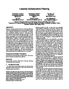
Figure 1 quantifies stability changes of matrix approximation method with the generalization error when rank r increases from 5 to 20. This experiment uses RSVD [35], a popular MA-based recommendation algorithm, on the MovieLens (1M) dataset (∼106 ratings, 6,040 users, 3,706 items). We choose in Definition 1 as 0.0046 to cover all error differences when r = 5. We compute

4

Percentage

100%

Stability vs. Gen Error

80% 60% 40% 20% 0% 0.03

0.06

0.09 0.12 RMSE Difference

0.15

Figure 1: Stability vs. generalization error with different rank r on the MovieLens (1M) dataset. ˆ ˆ Pr[|D(R)−D Ω (R)| < ] with 500 different runs to measure stability (y-axis), and compute RMSE differences between training and test data to measure generalization error (x-axis). As shown in Figure 1, the generalization error increases when rank r increases, because matrix approximation models become more complex and more biased on training data with higher ranks. In contrary, the stability of RSVD decreases when r increases. This indicates that (1) stability decreases when generalization error increases, and (2) RSVD cannot provide stable recommendation even when the rank is as low as 20. This study demonstrates that existing matrix approximation methods suffer from low generalization performance due to low algorithm stability. Therefore, it is important to develop stable matrix approximation methods with good generalization performance.

3

Stability of Matrix Approximation

In this section, we analyze the stability of matrix approximation in two different collaborative filtering tasks: 1) rating prediction and 2) top-N recommendation. We formally prove our key observations that introducing properly selected subsets into the loss functions can improve the stability of matrix approximation methods.

3.1

Stability Analysis of Matrix Approximation in the Rating Prediction Task

We first introduce the Hoeffding’s Lemma, and then analyze the stability properties of low-rank matrix approximation problems. Lemma 1 (Hoeffding’s Lemma). Let X bea real-valued random variable with zero mean and Pr (X ∈ [b, a]) = 1. Then, for any s ∈ R, E esX ≤ exp 18 s2 (a − b)2 . Following the Uniform Stability [4], given a stable matrix approximation algorithm, the approximation results remain stable if the change of the training data set, i.e., the set of observed entries Ω from the original matrix R, is small. For instance, we can remove a subset of easily predictable entries from Ω to obtain Ω0 . It is desirable that the solution of minimizing both DΩ and DΩ0 together will be more stable than the solution of minimizing DΩ only. The following Theorem 1 formally proves the statement.

5

Theorem 1. Let Ω (|Ω| > 2) be a set of observed entries in R. Let ω ⊂ Ω be a subset of observed ˆ i,j | ≤ DΩ (R). ˆ Let Ω0 = Ω − ω, then for any entries, which satisfies that ∀(i, j) ∈ ω, |Ri,j − R ˆ + λ1 DΩ0 (R) ˆ and DΩ (R) ˆ are δ1 -stable and > 0 and 1 > λ0 , λ1 > 0 (λ0 + λ1 = 1), λ0 DΩ (R) δ2 -stable, resp., then δ1 ≤ δ2 . ˆ − DΩ (R) ˆ ∈ [−a, a] (a = sup{D(R) ˆ − DΩ (R)}) ˆ ˆ − Proof. Let’s assume that D(R) and D(R) 0 0 0 ˆ ˆ ˆ ˆ ˆ (λ0 DΩ (R) + λ1 DΩ0 (R)) ∈ [−a , a ] (a = sup{D(R) − (λ0 DΩ (R) + λ1 DΩ0 (R))}) are two random variables with 0 mean. Based on Markov’s inequality, for any t > 0, we have ˆ ˆ ˆ − DΩ (R) ˆ ≥ ] ≤ E[exp (t(D(R) − DΩ (R)))] . Pr[D(R) exp (t) ˆ − DΩ (R)))] ˆ ˆ − Then, based on Lemma 1, we have E[exp (t(D(R) ≤ exp ( 21 t2 a2 ), i.e., Pr[D(R) 1 2 2 1 2 2 ˆ − DΩ (R) ˆ ≤ −] ≤ exp ( 2 t a ) . ˆ ≥ ] ≤ exp ( 2 t a ) . And similarly, we have Pr[D(R) DΩ (R) exp (t)

exp (t)

ˆ − DΩ (R)| ˆ ≥ ] ≤ Combining the two equations above, we have Pr[|D(R)

2 exp ( 21 t2 a2 ) exp (t) ,

i.e.,

1 2 2 ˆ − DΩ (R)| ˆ < ] ≥ 1 − 2 exp ( 2 t a ) . Pr[|D(R) exp (t)

(4)

Similarly, we have ˆ − (λ0 DΩ (R) ˆ + λ1 DΩ0 (R))| ˆ < ] ≥ 1 − Pr[|D(R)

2 exp ( 21 t2 a02 ) . exp (t)

(5)

We can compare a0 with a as follows: ˆ − DΩ (R) ˆ + λ1 (DΩ (R) ˆ − DΩ0 (R))} ˆ a0 = sup{D(R) ˆ − DΩ (R)} ˆ + λ1 sup{DΩ (R) ˆ − DΩ0 (R)} ˆ = sup{D(R) ˆ − DΩ0 (R)}. ˆ = a + λ1 sup{DΩ (R) 2 ˆ ˆ i,j | ≤ DΩ (R), ˆ we have 1/|ω| P ˆ 2 Since ∀(i, j) ∈ ω, |Ri,j − R (i,j)∈ω (Ri,j − Ri,j ) ≤ DΩ (R), ˆ ≤ DΩ (R). ˆ Then, since Ω = ω ∪ Ω0 , we have DΩ0 (R) ˆ ≥ DΩ (R). ˆ This means that i.e., Dω (R)

sup{DΩ (R) − DΩ0 (R)} ≤ 0. Thus, we have a0 ≤ a. Therefore, δ1 ≤ δ2 .

2 exp ( 21 t2 a02 ) exp (t)

≤

2 exp ( 12 t2 a2 ) exp (t) ,

i.e.,

Remark. Theorem 1 above indicates that, if we remove a subset of entries that are easier ˆ + λ1 DΩ0 (R) ˆ has a higher probability to predict than average from Ω to form Ω0 , then λ0 DΩ (R) ˆ ˆ ˆ ˆ will lead to of being close to D(R) than DΩ (R). Therefore, minimizing λ0 DΩ (R) + λ1 DΩ0 (R) ˆ solutions that have better generalization performance than minimizing DΩ (R). It should be noted ˆ i,j | ≤ DΩ (R) ˆ is not necessary. The conclusion will be that the condition that ∀(i, j) ∈ ω, |Ri,j − R ˆ ˆ the same if Dω (R) ≤ DΩ (R). The following Proposition 1 formally proves this. 6

Proposition 1. Let Ω (|Ω| > 2) be a set of observed entries in R. Let ω ⊂ Ω be a subset of ˆ ≤ DΩ (R). ˆ Let Ω0 = Ω − ω, then for any > 0 and observed entries, which satisfies that Dω (R) ˆ + λ1 DΩ0 (R) ˆ and DΩ (R) ˆ are δ1 -stable and δ2 -stable, 1 > λ0 , λ1 > 0 (λ0 + λ1 = 1), λ0 DΩ (R) resp., then δ1 ≤ δ2 . Proof. This proof is omitted as it is similar to that of Theorem 1. However, Theorem 1 and Proposition 1 only prove that it is beneficial to remove easily predictable entries from Ω to obtain Ω0 , but does not show how many entries should be removed from ˆ i,j | ≤ DΩ (R) ˆ Ω. The following Theorem 2 shows that removing more entries that satisfy |Ri,j − R 0 can yield better Ω . Theorem 2. Let Ω (|Ω| > 2) be a set of observed entries in R. Let ω2 ⊂ ω1 ⊂ Ω, and ω1 and ω2 ˆ i,j | ≤ DΩ (R). ˆ Let Ω1 = Ω − ω1 and Ω2 = Ω − ω2 , then for satisfy that ∀(i, j) ∈ ω1 (ω2 ), |Ri,j − R ˆ + λ1 DΩ (R) ˆ and λ0 DΩ (R) ˆ + λ1 DΩ (R) ˆ any > 0 and 1 > λ0 , λ1 > 0 (λ0 + λ1 = 1), λ0 DΩ (R) 1 2 are δ1 -stable and δ2 -stable, resp., then δ1 ≤ δ2 . ˆ − (λ0 DΩ (R) ˆ + λ1 DΩ (R)) ˆ ∈ [−a1 , a1 ] Proof. Similar to Theorem 1, let’s assume that D(R) 1 ˆ − (λ0 DΩ (R) ˆ + λ1 DΩ (R))}) ˆ ˆ − (λ0 DΩ (R) ˆ + λ1 DΩ (R)) ˆ ∈ [−a2 , a2 ] (a1 = sup{D(R) and D(R) 1 2 ˆ ˆ ˆ (a2 = sup{D(R) − (λ0 DΩ (R) + λ1 DΩ2 (R))}) are two random variables with 0 mean. Applying Lemma 1 and the Markov’s inequality, we have 1 2 2 ˆ − (λ0 DΩ (R) ˆ + λ1 DΩ (R))| ˆ < ] ≥ 1 − 2 exp ( 2 t a1 ) Pr[|D(R) 1 exp (t) 1 2 2 ˆ − (λ0 DΩ (R) ˆ + λ1 DΩ (R))| ˆ < ] ≥ 1 − 2 exp ( 2 t a2 ) . Pr[|D(R) 2 exp (t)

ˆ i,j | ≤ DΩ (R) ˆ and ω2 ⊂ ω1 , we have DΩ (R) ˆ ≤ DΩ (R). ˆ Thus, Since ∀(i, j) ∈ ω1 (ω2 ), |Ri,j − R 1 2 ˆ − DΩ (R)} ˆ ≤ 0. Since a1 = a2 + λ1 sup{DΩ (R) ˆ − DΩ (R)}, ˆ we have we have sup{DΩ1 (R) 2 1 2 a1 ≤ a2 . Then, similar to Theorem 1, we can conclude that δ1 ≤ δ2 . Remark. From Theorem 2, we know that removing more entries that are easy to predict will yield more stable matrix approximation. Therefore, it is desirable to choose Ω0 as the whole set of entries which are harder to predict than average, i.e., the whole set of entries satisfying ∀(i, j) ∈ Ω0 , ˆ i,j | ≥ DΩ (R). ˆ |Ri,j − R Theorem 1 and 2 only consider choosing one Ω0 to find stable matrix approximations. The next question is, is it possible to choose more than one Ω0 that satisfy the above condition, and yield more stable solutions by minimizing them all together. The following Theorem 3 shows that incorporating K such entry sets (Ω0 ) will be more stable than incorporating any K − 1 out of the K entry sets. Theorem 3. Let Ω (|Ω| > 2) be a set of observed entries in R. ω1 , ..., ωK ⊂ Ω (K > 1) satisfy ˆ i,j | ≤ DΩ (R). ˆ Let Ωk = Ω − ωk for all 1 ≤ k ≤ K. that ∀(i, j) ∈ ωk (1 ≤ k ≤ K), |Ri,j − R 7

P P ˆ ˆ Then, for any > 0 and 1 > λ0 , λ1 , ..., λK > 0 ( K i=0 λi = 1), λ0 DΩ (R) + k∈[1,K] λk DΩk (R) P ˆ ˆ + and (λ0 + λK )DΩ (R) k∈[1,K−1] λk DΩk (R) are δ1 -stable and δ2 -stable, resp., then δ1 ≤ δ2 . ˆ ˆ ˆ P ˆ Proof. Assume that D(R)−((λ 0 +λK )DΩ (R)+ k∈[1,K−1] λk DΩk (R)) ∈ [−a, a] (a = sup{D(R)− P P ˆ ˆ ˆ ˆ ˆ + ((λ0 + λK )DΩ (R) k∈[1,K] λk DΩk (R)) ∈ k∈[1,K−1] λk DΩk (R))} and D(R) − (λ0 DΩ (R) + P ˆ ˆ − (λ0 DΩ (R) ˆ + [−a0 , a0 ] (a0 = sup{D(R) k∈[1,K] λk DΩk (R))} are two random variables with 0 mean. Applying Lemma 1 and the Markov’s inequality, we have ˆ − (λ0 DΩ (R) ˆ + Pr[|D(R)

X k∈[1,K]

X

ˆ − ((λ0 + λK )DΩ (R) ˆ + Pr[|D(R)

k∈[1,K−1]

1 2 02 ˆ < ] ≥ 1 − 2 exp ( 2 t a ) λk DΩk (R))| exp (t)

2 exp ( 12 t2 a2 ) ˆ λk DΩk (R))| < ] ≥ 1 − . exp (t)

ˆ ˆ ≥ DΩ (R), ˆ which means sup{DΩ (R)−D ˆ Similar as the proofs above, we have DΩK (R) ΩK (R)} ≤ 0 0 ˆ ˆ 0. Since a = a + λK sup{DΩ (R) − DΩK (R)}, we know that a ≤ a. Thus, we can conclude that 2 exp ( 12 t2 a02 ) exp (t)

≤

2 exp ( 12 t2 a2 ) exp (t) ,

i.e., δ1 ≤ δ2 .

Remark. Theorem 3 shows that minimizing DΩ together with the RMSEs of more than one hard predictable subsets of Ω will help generate more stable matrix approximation solutions. However, sometimes it is expensive to find such “hard predictable subsets”, because we do not know which subset of entries to choose without any prior knowledge. Thus, we propose a solution to obtain hard predictable subsets of Ω based on only one set of easily predictable entries as follows: ˆ i,j | ≤ DΩ (R), ˆ and choose Ω0 = Ω − ω; 1) choose ω ⊂ Ω, which satisfies that ∀(i, j) ∈ ω, |Ri,j − R 2) divide ω into K non-overlapping subsets ω1 , ..., ωK with the condition that ∪k∈[1,K] ωk = ω, and ˆ to find ˆ + PK λk DΩ (R) choose Ωk = Ω − ωk for all 1 ≤ k ≤ K; and 3) minimize λ0 DΩ (R) k k=1 stable matrix approximation 4 proves that it is desirable to PK solutions.ˆ The following Theorem ˆ ˆ ˆ minimize λ0 DΩ (R) + k=1 λk DΩk (R) instead of λ0 DΩ (R) + (1 − λ0 )DΩ0 (R). Theorem 4. Let Ω (|Ω| > 2) be a set of observed entries in R. Choose ω ⊂ Ω, which satisfies ˆ i,j | ≤ DΩ (R). ˆ And divide ω into K non-overlapping subsets ω1 , ..., ωK that ∀(i, j) ∈ ω, |Ri,j − R with the condition that ∪k∈[1,K] ωk = ω. Let Ω0 = Ω − ω and Ωk = Ω − ωk for all 1 ≤ k ≤ K. P PK ˆ ˆ Then, for any > 0 and 1 > λ0 , λ1 , ..., λK > 0 ( K i=0 λi = 1), λ0 DΩ (R) + k=1 λk DΩk (R) ˆ ˆ and λ0 DΩ (R) + (1 − λ0 )DΩ0 (R) are δ1 -stable and δ2 -stable, resp., then δ1 ≤ δ2 . ˆ ˆ PK ˆ ˆ Proof. Let’s first assume that D(R)−(λ 0 DΩ (R)+ k=1 λk DΩk (R)) ∈ [−a1 , a1 ] (a1 = sup{D(R)− P K ˆ + ˆ ˆ ˆ ˆ (λ0 DΩ (R) k=1 λk DΩk (R))} and D(R) − (λ0 DΩ (R) + (1 − λ0 )DΩ0 (R)) ∈ [−a2 , a2 ] (a2 = ˆ − ((1 − λ0 )DΩ (R))} ˆ sup{D(R) are two random variables with 0 mean. 0 1 2 2 ˆ ˆ PK λk DΩ (R))| ˆ < ] ≥ 1− 2 exp ( 2 t a1 ) and Pr[|D(R)− ˆ We have Pr[|D(R)−(λ 0 DΩ (R)+ ˆ ((1 − λ0 )DΩ0 (R))| < ] ≥ 1 −

k=1 2 exp ( 21 t2 a22 ) exp (t) .

k

exp (t)

∀k ∈ [1, K] ωk ⊂ ω and ∀(i, j) ∈ ω, |Ri,j − 8

ˆ i,j | ≤ DΩ (R), ˆ we have for all k ∈ [1, K], DΩ ≤ DΩ . Sum the above inequation over all k ∈ R 0 k P P ˆ − (λ0 DΩ (R) ˆ + λk DΩ0 = (1 − λ0 )DΩ0 . Thus, sup{D(R) λk DΩk ≤ K [1, K], we have K k=1 k=1 PK ˆ ˆ ˆ k=1 λk DΩk (R))} ≤ sup{D(R) − ((1 − λ0 )DΩ0 (R))}, i.e., a1 ≤ a2 . Thus, we can conclude that δ1 ≤ δ2 . Remark. Theorem 4 shows that if we can find only one subset of entries that are easier to predict than average, then we can probe this subset of entries to increase the stability of matrix approximations.

3.2

Stability Analysis of Matrix Approximation in the General Setting

ˆ − DΩ (R) ˆ is within So far, all theoretical analysis rely on one key assumption: the value of D(R) ˆ ˆ a symmetric interval, e.g., [−a, a] (a = sup{D(R) − DΩ (R)}). The assumption holds for matrix approximation in the rating prediction tasks, but may not hold for all kinds of matrix approximation problems, e.g., binary matrix approximation for top-N recommendation. For instance, binary ˆ is typically matrix approximation typically minimizes “0-1” loss which is non-convex, so DΩ (R) defined as convex surrogate losses [44]. Apparently, the infimum and supremum of convex surˆ − DΩ (R) ˆ are not always symmetric around 0, e.g., the Exponential loss and Log rogated D(R) loss. For a more general case which holds for all kinds of matrix approximation problems, we only ˆ ˆ ˆ ˆ ˆ ˆ assume that E[D(R)−D Ω (R)] = 0, D(R)−DΩ (R) ∈ [b, a], where a = sup{D(R)−DΩ (R)} and ˆ − DΩ (R)}. ˆ The following theorem proves that we can derive matrix approximation b = inf{D(R) problems with higher stability by randomly choosing Ω0 ⊂ Ω with the above general assumption. Theorem 5. Let Ω (|Ω| > 2) be a set of observed entries in R and Ω0 ⊂ Ω be a randomly selected ˆ + subset of observed entries. Assume that, for any 1 > λ0 , λ1 > 0 (λ0 + λ1 = 1), λ0 DΩ (R) ˆ ˆ λ1 DΩ0 (R) and DΩ (R) are δ1 -stable and δ2 -stable, resp., then δ1 ≤ δ2 . Proof. Based on Markov’s inequality and Lemma 1, for any t > 0 and > 0, we have ˆ

1 2

ˆ

2

t(D(R)−DΩ (R)) ] e 8 t (a−b) ˆ − DΩ (R) ˆ ≥ ] ≤ E[e Pr[D(R) ≤ , et et ˆ − DΩ (R)} ˆ and b = inf{D(R) ˆ − DΩ (R)}. ˆ where a = sup{D(R) Based on Markov’s inequality and the convexity of exponential function, we have ˆ

ˆ

ˆ

E[et(D(R)−λ0 DΩ (R)−λ1 DΩ0 (R)) ] et ˆ ˆ ˆ ˆ t(λ (D( R)−D Ω (R))+λ1 (D(R)−DΩ0 (R))) ] E[e 0 = et ˆ ˆ ˆ ˆ λ0 E[et(D(R)−DΩ (R)) ] + λ1 E[et(D(R)−DΩ0 (R)) ] ≤ et 1 2 1 2 0 2 0 2 t (a−b) t e8 e 8 (a −b ) ≤ λ0 + λ . 1 et et

ˆ − λ0 DΩ (R) ˆ − λ1 DΩ0 (R) ˆ ≥ ] ≤ Pr[D(R)

9

ˆ − DΩ0 (R)} ˆ and b0 = inf{D(R) ˆ − where a and b are the same as above and a0 = sup{D(R) ˆ DΩ0 (R)}. Based on the properties of infimum and supremum, we have 2 ˆ − inf{D(R)}) ˆ ˆ − inf{DΩ (R)})) ˆ (a − b)2 = ((sup{D(R)} + (sup{DΩ (R)} 2 ˆ − inf{D(R)}) ˆ ˆ − inf{DΩ0 (R)})) ˆ (a0 − b0 )2 = ((sup{D(R)} + (sup{DΩ0 (R)}

ˆ ≤ sup{DΩ (R)} ˆ and inf{DΩ0 (R)} ˆ ≥ inf{DΩ (R)}, ˆ so Since Ω0 ⊂ Ω, we know that sup{DΩ0 (R)} ˆ − inf{DΩ0 (R)} ˆ ≤ sup{DΩ (R)} ˆ − inf{DΩ (R)}. ˆ that 0 ≤ sup{DΩ0 (R)} This will turn out that 0 0 2 2 (a − b ) ≤ (a − b) , which means 1 2 (a−b)2

λ0

e8t

et

1 2 0 (a −b0 )2

+ λ1

e8t

et

1 2 (a−b)2

≤

e8t

et

.

Based on the above inequality, we can conclude that δ1 ≤ δ2 . Remark. Theorem 5 above indicates that, if we randomly choose a subset of entries from Ω to ˆ ˆ ˆ form Ω0 , then λ0 DΩ (R)+λ 1 DΩ0 (R) will also have a higher probability of being close to D(R) than ˆ Therefore, minimizing λ0 DΩ (R) ˆ + λ1 DΩ0 (R) ˆ is more desirable than minimizing DΩ (R). ˆ DΩ (R). ˆ Note that, as shown in the proof, the sharpness of the stability bound depends on sup{DΩ0 (R)} ˆ However, it is non-trivial to directly infer sup{DΩ0 (R)} ˆ and inf{DΩ0 (R)} ˆ from and inf{DΩ0 (R)}. 0 0 a randomly chosen Ω . In this case, Ω should be considered as a tunable parameter in practice. A better choice of Ω0 will yield sharper stability bound and thus yield better model performance. Similarly, we can also select subsets from Ω0 and form optimization problems that are even ˆ + λ1 DΩ0 (R). ˆ The following theorems formally prove this idea. more stable than λ0 DΩ (R) Theorem 6. Let Ω (|Ω| > 2) be a set of observed entries in R. Let Ω1 ⊂ Ω2 ⊂ ... ⊂ ΩK ⊂ Ω (K > 1) be randomly selected subsets ofP observed entries. Assume that, for any 1 > λ0 , λ1 , ..., λK > 0 P K ˆ ˆ ˆ λ = 1), λ D ( R) + (λ0 + K 0 Ω s=1 λs DΩs (R) and DΩ (R) are δ1 -stable and δ2 -stable, resp., s=1 s then δ1 ≤ δ2 . Proof. This proof is omitted as it is similar to that of Theorem 5. Similarly, we can also select K different random subsets to further improve the stability of matrix approximation, which is formally described in the following Theorem 7. Theorem 7. Let Ω (|Ω| > 2) be a set of observed entries in R. Let Ω1 Ω2 , ..., ΩK P(K > 1) be randomly selected subsets of Ω.. Assume that, for any 1 > λ0 , λ1 , ..., λK > 0 (λ0 + K s=1 λs = 1), PK ˆ ˆ ˆ λ0 DΩ (R) + s=1 λs DΩs (R) and DΩ (R) are δ1 -stable and δ2 -stable, resp., then δ1 ≤ δ2 . Proof. This proof is omitted as it is similar to that of Theorem 5. Remark. Theorem 6 and Theorem 7 above indicate that, if we randomly choose different subsets of entries from Ω, then we can obtain even more stable optimization problems than only 10

choosing one Ω0 . The performance of adopting Theorem 6 will be influenced by the selection of the largest subset (ΩK ) because all the other subsets depend on it. Therefore, a bad selection of ΩK will not significantly improve the stability. But the selected subsets are independent in Theorem 7. As such, a few bad selections will not significantly affect the performance. Therefore, it will be more desirable to adopt Theorem 7 than Theorem 6 if there is no clear clue to select proper subsets.

4

Stable Matrix Approximation Algorithm for Collaborative Filtering

This section first presents the stable matrix approximation (SMA) method for the rating prediction task, and then presents stable matrix approximation for the top-N recommendation task. Finally, we present how to solve the algorithm stability optimization problem using a stochastic gradient descent method.

4.1

SMA for Rating Prediction

In the rating prediction task, the goal of stable matrix approximation-based q P collaborative filtering 1 ˆ ˆ 2 is to minimize the root mean square error (RMSE), i.e., DΩ (R) = |Ω| (i,j)∈Ω (Ri,j − Ri,j ) . Here, we present the stable matrix approximation algorithm in terms of RMSE. 4.1.1

Model Formulation

Singular value decomposition (SVD) is one of the commonly used methods for matrix approximation in the rating prediction task [6]. Based on the analysis of stable matrix approximation described in the previous section, it is desirable to minimize the loss functions that will lead to solutions with good generalization performance. Let {Ω1 , ..., ΩK } be subsets of Ω which satisfy that ∀s ∈ [1, K], DΩs ≥ DΩ . Then, following Theorem 4, we propose a new extension of SVD. Note that, extensions to other matrix approximation methods can be similarly derived. ˆ = arg min λ0 DΩ (X) + R X

K X

λs DΩs (X)

s=1

s.t. rank(X) = r.

(6)

where λ0 , λ1 , ..., λK define the contributions of each component in the loss function. 4.1.2

Hard Predictable Subsets Selection

The key step in Equation 6 is to obtain subsets of Ω — {Ω1 , ..., ΩK } which satisfy that ∀s ∈ [1, K], DΩs ≥ DΩ . To obtain such Ωs is not trivial, because we can only check if the condition is satisfied with the final model. But the final model cannot be known before we define and optimize a given loss function. 11

First, we propose the following idea to address this issue: 1) approximate the target matrix R with existing matrix approximation solutions, e.g., RSVD [35]; 2) choose each entry (i, j) ∈ ˆ i,j | < DΩ and small probability otherwise; and 3) obtain Ω with high probability if |Ri,j − R 0 Ω by removing the chosen entries to satisfy the condition of Proposition 1, or probe Ω0 to find hard predictable subsets that satisfy the condition of Theorem 4. By assuming that other matrix approximation methods will not dramatically differ from the final model of SMA, we can ensure that Ω0 will satisfy DΩ0 ≥ DΩ with high probability.

4.2

SMA Algorithm for Top-N Recommendation

In the top-N recommendation task, the goal of stable matrix approximation is to minimize the “01 P ˆ 1” error as in classification tasks [41], i.e., DΩ = |Ω| (i,j)∈Ω 1(Ri,j , Ri,j ) where 1(x, y) is an indicator function. 1(x, y) = 1 if x = y, and 1(x, y) = 0 otherwise. Here, we present the stable matrix approximation algorithm based on the above “0-1” loss. 4.2.1

Loss Functions

Since the original “0-1” loss is not differentiate, gradient-based learning algorithms, e.g., SGD, cannot be applied to learn the models. Therefore, surrogate loss functions are commonly adopted to define convex losses. The following popular surrogate loss functions [32, 24] are adopted in ˆ i,j , Ri,j ) = (R ˆ i,j − Ri,j )2 ; 2) log loss (Log): this paper: 1) mean square error (MSE): LM SE (R ˆ i,j , Ri,j ) = log(1 + exp{−R ˆ i,j Ri,j }); and 3) exponential loss (Exp): LExp (R ˆ i,j , Ri,j ) = LLog (R ˆ i,j Ri,j }. After introducing surrogate loss functions, the new loss function of SMA for exp{−R top-N recommendation can be defined as follows: DΩ =

1 X ˆ i,j ) L∗ (Ri,j , R |Ω|

(7)

(i,j)∈Ω

where L∗ can be any of the surrogate loss functions. The new loss function is convex because the surrogate loss functions are convex, so that it can be optimized using gradient-based learning algorithms such as SGD. In real-world top-N recommendation tasks, the positive ratings are very limited, which causes severe data imbalance issue. To address this issue, weighting is adopted by many matrix approximation methods [15, 14] as follows: DΩ =

1 X ˆ i,j ) Wi,j L∗ (Ri,j , R |Ω|

(8)

(i,j)∈Ω

where Wi,j is the weight for entry (i, j). Typically, Wi,j is set to a large value when Ri,j = 1 and a small value when Ri,j = −1. In this paper, we fix the weights for positive and negative examples for simplicity of analysis, i.e., we use a universal weight for all positive examples and another universal weight for all negative examples. Recent works [15, 14] have proved that weighed matrix 12

approximation methods can improve accuracy of top-N recommendation on implicit feedback data. Similarly, we can extend matrix approximation with the weighted loss above to generate a stable matrix approximation method as in Equation 6. 4.2.2

Subset Selection

Similar to the rating prediction task, subsets of Ω should be selected to improve the stability of learned MA models for top-N recommendation. According to Theorem 5, we can randomly choose Ω0 and optimize the following problem with better stability: ˆ = arg min λ0 DΩ (X) + λ1 DΩ0 (X) R X

s.t. rank(X) = r.

(9)

However, a random Ω0 could improve stability, but it may also hurt optimization accuracy (training accuracy). Therefore, the test accuracy may not be improved. To further improve the stability of learned models without much degradation in optimization accuracy, it is more desirable to select Ω0 as the hard-predictable subsets, because hard-predictable subsets have tighter gap between infimum and supremum, i.e., can achieve smaller δ in the stability measure. For top-N recommendation, we can assume that examples near the decision boundary are harder to predict than others. Then, we can select Ω0 as follows: ˆ i,j ∈ [−γ, γ]}. Ω0 = {(i, j) : R (10) where γ > 0 defines the margin to select the examples. The above definition means that entry (i, j) will be selected in Ω0 if its predicted rating is near 0. Then, for the t-th epoch, we can easily select Ω0 based on the model output at the t − 1-th epoch. 4.2.3

Discussion

In SMA for top-N recommendation, we change the original “0-1” loss to surrogate losses and adopt weighting to give higher weights to rare positive examples. Here, we show that the stability analysis from Theorem 5 to Theorem 7 can still be applied to the surrogated and weighted loss functions. Assuming that the entries in Ω are independently and identically selected from its distribution, we can know that the ratio between positive examples and negative examples is the same for Ω and ˆ − DΩ (R)] ˆ = 0, which means that the the whole set of examples. Then, we can know that E[D(R) precondition of Theorem 5 to Theorem 7 holds. Therefore, we can apply the stability analysis in these theorems in SMA for top-N recommendation task as described above.

4.3

The SMA Learning Algorithm

Algorithm 1. shows the pseudo-code of the proposed SMA learning algorithm to solve the optimization problem defined in Equation 6 by adopting hard predictable subsets. From Step 1 to 9, we obtain K different hard predictable entry sets. Note that, for top-N recommendation, hard 13

Algorithm 1 The SMA Learning Algorithm ˆ is an approximation of R Require: R is the targeted matrix, Ω is the set of entries in R, and R by existing matrix approximation methods. p > 0.5 is the predefined probability for entry selection. µ1 and µ2 are the coefficients for L2-regularization. 1: Ω0 = ∅; 2: for each (i, j) ∈ Ω do 3: randomly generate ρ ∈ [0, 1]; ˆ i,j | ≤ DΩ & ρ ≤ p) or (|Ri,j − R ˆ i,j | > DΩ & ρ ≤ 1 − p) then 4: if (|Ri,j − R 0 0 5: Ω ← Ω ∪ {(i, j)}; 6: end if 7: end for 0 8: randomly divide Ω0 into ω1 , ..., ωK (∪K k=1 ωi = Ω ); 9: for all k ∈ [1, K], Ωk = Ω − ωk ; ˆ , Vˆ ) : = arg minU,V [PK λk DΩ (U T V ) +λ0 DΩ (U V T ) + µ1 k U k2 +µ2 k V k2 ] 10: (U k k=1 ˆ=U ˆ Vˆ T 11: return R predictable subsets can be selected by Equation 10. In Step 10, the optimization is performed by stochastic gradient descent (SGD), the details of which are trivial and thus omitted here. Also, L2 regularization is adopted in Step 10. Note that, other types of optimization methods and regularization techniques can also be used in Algorithm 1. The complexity of Step 1 to 9 is O(|Ω|) for the rating prediction task and O(mn) for the top-N recommendation task, where |Ω| is the number of observed entries in R and m, n is the matrix size. The complexity of Step 10 is O(rmn) per-iteration, where r is the rank and m, n is the matrix size. Thus, the computation complexity of SMA is similar to that of classic matrix approximation methods, such as regularized SVD [35].

5

Experiments

In this section, we first introduce the experimental setup, including dataset description, parameter setting, evaluation metrics and compared methods. Then, we analyze the performance of SMA for the rating prediction task from the following aspects: 1) generalization performance of SMA; 2) sensitivity of SMA with different parameters, e.g., rank r and the number of non-overlapping subsets K; 3) accuracy comparison between SMA and seven state-of-then-art matrix approximation based recommendation algorithms, including four single MA methods and three ensemble methods; and 4) SMA’s accuracy in different data sparsity settings. After that, we analyze the performance of SMA for the top-N recommendation task from the following aspects: 1) generalization performance of SMA; 2) sensitivity of SMA with different parameters, e.g., surrogate loss functions and γ values; and 3) accuracy comparison between SMA and four state-of-the-art top-N recommendation algorithms.

14

5.1

Experimental Setup

Data Description. Four popular datasets are adopted to evaluate SMA: 1) MovieLens1 100K (943 users, 1682 movies, 105 ratings); 2) MovieLens 1M (∼6k users, 4k items, 106 ratings); 3) MovieLens 10M (∼70k users, 10k items, 107 ratings) and 4) Netflix (∼480k users, 18k items, 108 ratings). These datasets are rating-based, so we follow other works [37, 33] to transform the data to binary data for the top-N recommendation task in which the models predict whether a user will rate an item or not. For each dataset, we randomly split it into training and test sets and keep the ratio of training set to test set as 9:1. All experimental results are presented by averaging the results over five different random train-test splits. Parameter Setting. For the rating prediction task, we use learning rate v = 0.001 for stochastic gradient decent, µ1 = 0.06 for L2 -regularization coefficient, = 0.0001 for gradient descent convergence threshold, and T = 250 for maximum number of iterations. For the top-N recommendation task, we use learning rate v = 0.001 for stochastic gradient decent, µ1 = 0.001 for L2 regularization coefficient, = 0.0001 for gradient descent convergence threshold, and T = 2000 for maximum number of iterations. Optimal parameters of the compared methods are chosen from their original papers. Note that adaptive learning rate methods, e.g., AdaError [27], can be adopted to further improve the accuracy of the proposed method. Evaluation Metrics. Theqaccuracy of rating prediction is evaluated using root mean square er1 P ˆ 2 ror (RMSE) as follows: (i,j)∈Ω (Ri,j − Ri,j ) . The accuracy of top-N recommendation |Ω| is evaluated using Precision and normalized discounted cumulative gain (NDCG) as follows: 1) Precision@N for a targeted user u can be computed as follows: P recision@N = |Ir ∩ Iu |/|Ir | where Ir is the list of top N recommendations and Iu is the list of items that u is interested in and 2) NDCG@N for a targeted P user u can be computed as follows: N DCG@N = DCG@N/IDCG@n, where DCG@N = nk=1 (2reli − 1)/log2 (i + 1) and IDCG@n is the value of DCG@N with perfect ranking (reli = 1 if u is interested to the i-th recommendation and reli = 0 otherwise). Compared Methods. For rating prediction task, we compare the performance of SMA with four single matrix approximation methods and three ensemble matrix approximation methods as follows: • Regularized SVD [35] is a popular matrix factorization method, in which user/item features are estimated by minimizing the sum-squared error using L2 regularization. • BPMF [39] is a Bayesian extension of PMF with model parameters and hyperparameters estimated using Markov chain Monte Carlo method. • APG [43] computes the approximation by solving a nuclear norm regularized linear least squares problem to speed up convergence. • GSMF [46] can transfer information among multiple types of user behaviors by modeling the shared and private latent factors with group sparsity regularization. • DFC [31] is an ensemble method, which divides a large-scale matrix factorization task into smaller subproblems, solves each other in parallel, and finally combines the subproblem solutions 1

https://grouplens.org/datasets/movielens/

15

to improve accuracy. • LLORMA [25] is an ensemble method, which assumes that the original matrix is described by multiple low-rank submatrices constructed by non-parametric kernel smoothing techniques. • WEMAREC [9] is an ensemble method, which constructs biased model by weighting strategy to address the insufficient data issue in each submatrix and integrates different biased models to achieve higher accuracy. For top-N recommendation, we compare SMA with the following four state-of-the-art collaborative filtering methods: • WRMF [15] assigns point-wise confidences to different ratings so that positive examples will have much larger confidence than negative examples. • BPR [37] minimizes a pair-wise loss function to optimize ranking measures, e.g., NDCG. They proposed different versions of BPR methods, e.g., BPR-kNN and BPR-MF. We compare SMA with the BPR-MF, which is also MA-based recommendation method; • AOBPR [36] improves the original BPR method by a non-uniform item sampler and meanwhile oversamples informative pairs to speed up convergence. • SLIM [33] generates top-N recommendations by aggregating user rating profiles using sparse representation. In their method, the weight matrix of user ratings is obtained by solving an L1 and L2 regularized optimization problem.

5.2 5.2.1

Rating Prediction Evaluation Generalization Performance MovieLens 10M RSVD(train set) RSVD(test set) SMA(train set) SMA(test set)

0.95

RMSE

0.90 0.85 0.80 0.75 0.70 0.65 0

20

40

60

80

100 120 140 160 180

Epochs

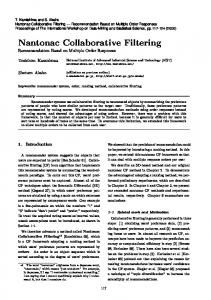
Figure 2: Training and test errors vs. epochs of RSVD and SMA on the MovieLens 10M dataset. Figure 2 compares training/test errors of SMA and RSVD with different epochs on the MovieLens 10M dataset (rank r = 20 and subset number K = 3). As we can see, the differences between training and test error of SMA are much smaller than that of RSVD. Moreover, the training error and test error are very close when epoch is less than 100. This result demonstrates that SMA can 16

indeed find models that have good generalization performance and yield small generalization error during the training process. 5.2.2

Sensitivity Analysis MovieLens 10M

Netflix

0.84 0.86

RMSE

0.82

0.80

RMSE

RSVD BPMF APG GSMF DFC LLORMA WEMAREC SMA


0.84

0.82

0.78 0.80 1

2

3 #Subsets

4

5

1

2

3 #Subsets

4

5

Figure 3: Effect of subset number K on the MovieLens 10M dataset (left) and Netflix dataset (right). SMA models are indicated by solid lines and other compared methods are indicated by dotted lines. MovieLens 10M

Netflix

0.84

0.87

0.83

0.86

RMSE

0.81 0.80 0.79


0.85 RMSE


0.82

0.84 0.83 0.82

0.78

0.81

0.77 0.80 50

100

150 Rank

200

250

50

100

150 Rank

200

250

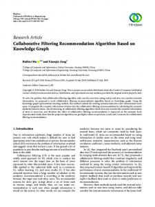
Figure 4: Effect of rank r on the MovieLens 10M dataset (left) and Netflix dataset (right). SMA and RSVD models are indicated by solid lines and other compared methods are indicated by dotted lines. Figure 3 investigates how SMA performs by varying number of non-overlapping subsets K (rank r = 200) and the optimal RMSEs of all compared methods on both Movielens 10M (left) and Netfilx (right) datasets. As we can see, SMA outperforms all these state-of-the-art methods with K varying from 1 to 5. It should be noted that, when K = 0, SMA is degraded to RSVD. Thus, the fact that SMA can produce better recommendations than RSVD confirms Theorem 1: with 17

Table 1: RMSEs of SMA and the seven compared methods on MovieLens (10M) and Netflix datasets. MovieLens (10M) Netflix RSVD 0.8256 ± 0.0006 0.8534 ± 0.0001 BPMF 0.8197 ± 0.0004 0.8421 ± 0.0002 APG 0.8101 ± 0.0003 0.8476 ± 0.0003 GSMF 0.8012 ± 0.0011 0.8420 ± 0.0006 DFC 0.8067 ± 0.0002 0.8453 ± 0.0003 LLORMA 0.7855 ± 0.0002 0.8275 ± 0.0004 WEMAREC 0.7775 ± 0.0007 0.8143 ± 0.0001 SMA 0.7682 ± 0.0003 0.8036 ± 0.0004 P ˆ additional terms K s=1 λs DΩs (R), we can improve the stability of MA models. In addition, we can see that the RMSEs on both datasets decrease as K increases. This further confirms Theorem 4: probing easily predictable entries to form harder predictable entry sets can better increase the model performance. Figure 4 analyzes the effect of rank r on MovieLens 10M (left) and Netflix (right) datasets by fixing K = 3. It can be seen that for any rank r from 50 to 250, SMA always outperforms the other seven compared methods in recommendation accuracy. And higher ranks for SMA will lead to better accuracy when the rank r increases from 50 to 250 on both two datasets. It is interesting to see that the recommendation accuracies of RSVD decrease slightly when r > 50 due to over-fitting and SMA can consistently increase recommendation accuracy even when r > 200. This indicates that SMA is less prone to over-fitting than RSVD, i.e., SMA is more stable than RSVD. 5.2.3

Accuracy Comparisons

Table 1 presents the performance of SMA with rank r = 200 and subset number K = 3. The compared methods are as follows: RSVD (r = 50) [35], BPMF (r = 300) [39], APG (r = 100) [43], GSMF (r = 20) [46], DFC (r = 30) [31], LLORMA (r = 20) [25] and WEMAREC (r = 20) [9] on MovieLens 10M and Netflix datasets. Notably, DFC, LLORMA and WEMAREC are ensemble methods, which have been shown to be more accurate than single methods due to better generalization performance. However, as shown in Table 1, our SMA method significantly outperforms all seven compared methods on both two datasets. This confirms that SMA can indeed achieve better generalization performance than both state-of-the-art single methods and ensemble methods. The main reason is that SMA can minimize objective functions that lead to solutions with good generalization performance, but other methods cannot guarantee low gap between training error and test error.

18

MovieLens 10M 1.05 RSVD(r=50) BPMF(r=50) APG(r=50) GSMF(r=50) SMA(r=50)

RMSE

1.00 0.95 0.90 0.85 0.80 20%

40%

60%

80%

Traning Set Ratio

Figure 5: RMSEs of SMA and four single methods with varying training set size on the MovieLens 10M dataset (rank r = 50). 5.2.4

Performance under Data Sparsity

Figure 5 presents the RMSEs of SMA vs. the training set size as compared with four single LRMA methods (RSVD, BPMF, APG and GSMF). The rank r of all five methods are fixed to 50. Note that, the rating density becomes more sparse when the training set ratio decreases. The results show that all methods can improve accuracy when the training set size increases, but the proposed SMA method always outperforms the other methods. This demonstrates that SMA can still provide stable matrix approximation even on very sparse dataset.

Top-N Recommendation Evaluation

5.3.1 1.00

Generalization Performance 1.00

WMA (train set) WMA (test set)

1.00

SMA rand (train set) SMA rand (test set)

0.80 Precision@10

Precision@10

0.80 0.60 0.5593 0.40 0.20

0.60 0.5454 0.40 0.20

0.00 200

300 Epochs

400

500

0.60 0.5534 0.40 0.20

0.00 100

SMA (train set) SMA (test set)

0.80 Precision@10

5.3

0.00 100

200

300 Epochs

400

500

100

200

300 Epochs

400

500

Figure 6: Generalization performance analysis of SMA with weighted Exp loss on MovieLens 100K dataset. The leftmost figure shows a weighted MA (WMA) methods without selecting Ω0 , which is equivalent to SMA with Ω0 = ∅. The middle figure shows SMA with random selected Ω0 . The rightmost figure shows SMA with hard predictable Ω0 , i.e., examples with predicted ratings in [-0.3,0.3] are selected as Ω0 .

19

Figure 6 compares the generalization performance of three different matrix approximation methods in the top-N setting: 1) weighted matrix approximation (WMA), which is the same as SMA except that WMA has no additional terms in the loss function, i.e., WMA learns MA models by optimizing Equation 8; 2) stable matrix approximation with random Ω0 (SMA rand), in which Ω0 is randomly selected rather than selecting the examples near the decision boundary; and 3) stable matrix approximation, in which Ω0 is selected as the examples near the decision boundary. As shown in Figure 6, both SMA rand and SMA can achieve lower gap between training precision@10 and test precision@10 than WMA, which confirms with Theorem 5: adding the term DΩ0 in the loss function can improve the stability of MA models, i.e., improve the generalization performance. For SMA rand, we can see that, although its generalization performance improves, its optimization performance (training accuracy) is affected due to the random selection of Ω0 . This demonstrates that random selection of Ω0 can improve generalization performance but degrade optimization performance simultaneously. Therefore, the test accuracy of SMA rand has no improvement compared with WMA. For SMA with hard predictable Ω0 , the optimization performance (training accuracy) is not affected but improved compared with WMA. This is because examples near the decision boundary are given larger gradients updates in SMA, which can help improve the optimization performance because examples near the decision boundary have higher optimization error. Meanwhile, compared with WMA, the generalization performance of SMA is also improved, which is due to the stability improvement from the selection of Ω0 . Since both the optimization performance and generalization performance are improved in SMA for top-N recommendation, SMA achieves significantly higher test accuracy than WMA. This experiment demonstrates that selecting random subsets can improve generalization performance but cannot improve test accuracy due to the degradation of training accuracy. On the contrary, adding properly selected subsets, e.g., examples near the decision boundary, can improve generalization performance and does not hurt training accuracy, and can thus improve test accuracy. 5.3.2

Sensitivity of Surrogate Losses

1.00

0.80

0.80

0.60 SMA-MSE (train set) SMA-MSE (test set) 0.40

Precision@10

0.60 Precision@10

Precision@10

0.80

1.00

SMA-Log (train set) SMA-Log (test set)

0.40

0.20

0.20 0.00 500

1000 Epochs

1500

2000

SMA-Exp (train set) SMA-Exp (test set) 0.40 0.20

0.00 0

0.60

0.00 0

500

1000 Epochs

1500

2000

0

200

400 600 Epochs

800

1000

Figure 7: Comparison of SMA with different surrogate losses on the MovieLens 100K dataset. Here, we choose γ = 0.3 and rank r = 100. Figure 7 compares the performance of SMA with three different surrogate loss functions: 1) mean square error (MSE); 2) log loss (Log) and 3) exponential loss (Exp). As shown in Figure 7, 20

SMA with mean square loss achieves much worse test accuracy compared with SMA with log loss and exponential loss, which is because mean square loss is a rating-based loss rather than a ranking-based loss. SMA with log loss and exponential loss achieve very similar test accuracy. However, the convergence speed of SMA with exponential loss is much faster (around 500 epochs) than that of SMA with log loss (around 2000 epochs). Therefore, SMA with exponential loss is more desirable due to decent accuracy and faster convergence speed. 5.3.3

Accuracy vs. γ 1

SMA Fraction of examples

Precision@10

0.24

0.23

0.22 0.1

0.3

0.5

0.7

SMA (γ=0.1) SMA (γ=0.3) SMA (γ=0.5) SMA (γ=0.7) SMA (γ=0.9)

0.8 0.6 0.4 0.2 0

0.9

0

γ

200

400 600 Epochs

800

1000

Figure 8: Accuracy vs. γ values of SMA on MovieLens 100K dataset. The figure on the left shows how the Precision@10 varies as γ changes from 0.1 to 0.9, and the figure on the right shows the ratio of selected examples in Ω0 with different γ values. Figure 8 compares the performance of SMA with different γ values, in which training examples with predicted ratings ranging in [−γ, γ] are selected as Ω0 for each epoch. The figure on the left shows how the recommendation accuracy varies as γ increases from 0.1 to 0.9, and the figure on the right shows the ratio of selected examples in Ω0 with different γ values. As shown in Figure 8, SMA with γ = 0.3 achieves the best test accuracy. For smaller γ, e.g., 0.1, or larger γ, e.g., 0.9, SMA achieves worse accuracy because too small or too large fraction of examples are chosen in Ω0 . This further confirms that the accuracy of SMA will vary with different Ω0 and properly selected Ω0 can help achieve better accuracy. 5.3.4

Accuracy Comparison

Table 2 and Table 3 compare SMA’s accuracy in top-N recommendation (Precision@N and NDCG@N) with one rating-based MA method (RSVD) and four state-of-the-art top-N recommendation methods (BPR, WRMF, AOBRP, SLIM) on the Movielens 1M and Movielens 100K datasets. Among the compared methods, RSVD is a baseline method, which aims at minimizing rating-based error. WRMF, BPR and AOBPR are matrix approximation-based collaborative filtering methods for

21

Table 2: Precision comparison between SMA and one rating-based MA method (RSVD) and four state-of-the-art top-N recommendation methods (BPR, WRMF, AOBRP, SLIM) on the Movielens 1M and Movielens 100K datasets. Bold face means that SMA statistically significantly outperforms the other methods with 95% confidence level.

ML-100K

ML-1M

Metric Data | Method RSVD BPR WRMF AOBPR SLIM SMA RSVD BPR WRMF AOBPR SLIM SMA

N=1 0.1659 ± 0.0017 0.3062 ± 0.0030 0.2761 ± 0.0074 0.3098 ± 0.0076 0.3053 ± 0.0097 0.5133 ± 0.0047 0.3155 ± 0.0038 0.3439 ± 0.0168 0.3851 ± 0.0116 0.3395 ± 0.0099 0.3951 ± 0.0056 0.4179 ± 0.0072

Precision@N N=5 N=10 0.1263 ± 0.0005 0.1037 ± 0.0009 0.2277 ± 0.0074 0.1896 ± 0.0048 0.2155 ± 0.0009 0.1816 ± 0.0007 0.2315 ± 0.0002 0.1926 ± 0.0022 0.2208 ± 0.0039 0.1836 ± 0.0006 0.3937 ± 0.0064 0.3258 ± 0.0061 0.2179 ± 0.0007 0.1403 ± 0.0035 0.2533 ± 0.0082 0.2061 ± 0.0040 0.2752 ± 0.0053 0.2202 ± 0.0056 0.2591 ± 0.0057 0.2119 ± 0.0031 0.2625 ± 0.0090 0.2055 ± 0.0031 0.2931 ± 0.0023 0.2347 ± 0.0033

N=20 0.0766 ± 0.0020 0.1516 ± 0.0007 0.1459 ± 0.0004 0.1540 ± 0.0016 0.1419 ± 0.0029 0.2548 ± 0.0051 0.1300 ± 0.0057 0.1581 ± 0.0028 0.1679 ± 0.0035 0.1632 ± 0.0025 0.1539 ± 0.0015 0.1772 ± 0.0022

top-N recommendation. SLIM is not an MA-based method, but we compare with it due to its superior accuracy in the top-N recommendation task. Here, we choose exponential loss for SMA with boundary margin γ = 0.3, rank r = 200, λ0 = λ1 = 1, Wi,j = 1 for positive ratings and Wi,j = 0.03 for negative ratings. As shown in the results, SMA consistently and significantly outperforms all the five compared methods on both datasets in terms of Precision@N and NDCG@N with N varying from 1 to 20. This is because all the other methods do not consider generalization performance but only optimization performance in model learning, which cannot ensure optimal test accuracy due to low generalization performance. Note that WRMF can be regarded as a special case of SMA if we adopt mean square surrogate loss and do not add subset to improve stability for SMA. Similar to the previous experiments, SMA significantly outperforms WRMF, which further confirms that introducing properly selected subset can improve the accuracy of collaborative filtering in the top-N recommendation task.

6

Related Work

Algorithmic stability has been analyzed and applied in several popular problems, such as regression [4], classification [4], ranking [21], marginal inference [30], etc. [4] first proposed a method of obtaining bounds on generalization errors of learning algorithms, and formally proved that regular-

22

Table 3: NDCG comparison between SMA and one rating-based MA method (RSVD) and four state-of-the-art top-N recommendation methods (BPR, WRMF, AOBRP, SLIM) on the Movielens 1M and Movielens 100K datasets. Bold face means that SMA statistically significantly outperforms the other methods with 95% confidence level.

ML-100K

ML-1M

Metric Data | Method RSVD BPR WRMF AOBPR SLIM SMA RSVD BPR WRMF AOBPR SLIM SMA

N=1 0.0324 ± 0.0020 0.0538 ± 0.0006 0.0510 ± 0.0013 0.0532 ± 0.0018 0.0551 ± 0.0015 0.0729 ± 0.0007 0.0389 ± 0.0028 0.0783 ± 0.0036 0.0913 ± 0.0034 0.0770 ± 0.0043 0.0912 ± 0.0021 0.1013 ± 0.0041

NDCG@N N=5 N=10 0.0700 ± 0.0006 0.0864 ± 0.0002 0.1235 ± 0.0003 0.1601 ± 0.0035 0.1202 ± 0.0002 0.1563 ± 0.0013 0.1200 ± 0.0006 0.1567 ± 0.0009 0.1201 ± 0.0023 0.1586 ± 0.0028 0.1758 ± 0.0021 0.2346 ± 0.0034 0.1047 ± 0.0032 0.0996 ± 0.0059 0.1803 ± 0.0056 0.2351 ± 0.0056 0.1989 ± 0.0030 0.2535 ± 0.0045 0.1801 ± 0.0044 0.2343 ± 0.0051 0.1967 ± 0.0036 0.2476 ± 0.0050 0.2136 ± 0.0050 0.2708 ± 0.0052

N=20 0.1006 ± 0.0001 0.2070 ± 0.0011 0.2012 ± 0.0010 0.2021 ± 0.0009 0.1948 ± 0.0043 0.3002 ± 0.0048 0.1393 ± 0.0071 0.2929 ± 0.0065 0.3131 ± 0.0043 0.2930 ± 0.0058 0.3017 ± 0.0091 0.3321 ± 0.0056

ization networks posses the uniform stability property. Then, [5] extends the algorithmic stability concept from regression to classification. [20] generalized the work of [4] and proposed the notion of training stability, which can ensure good generalization error bounds even when the learner has infinite VC dimension. [21] proposed query-level stability and gave query-level generalization bounds to learning to rank algorithms. [2] derived generalization bounds for ranking algorithms that have good properties of algorithmic stability. [40] considered the general learning setting including most statistical learning problems as special cases, and identified that stability is the necessary and sufficient condition for learnability. [30] proposed the concept of collective stability for structure prediction, and established generalization bounds for structured prediction. This work differs from the above works in that (1) this work introduces the stability concept to matrix approximation problem, and proves that matrix approximations with high stability will have high probability to generalize well and (2) most existing works focus on theoretical analysis, but this work provides a practical framework for achieving solutions with high stability. Matrix approximation methods have been extensively studied recently in the context of collaborative filtering. [23] analyzed the optimization problems of Non-negative Matrix Factorization (NMF). [42] proposed Maximum-Margin Matrix Factorization (MMMF), which can learn lownorm factorizations by solving a semi-definite program to achieve collaborative prediction. [38] viewed matrix factorization from a probabilistic perspective and proposed Probabilistic Matrix Factorization (PMF). Later, they proposed Bayesian Probabilistic Matrix Factorization (BPMF) [39] by giving a fully Bayesian treatment to PMF. [22] also extends PMF and developed a non-linear PMF 23

using Gaussian process latent variable models. [35] applied regularized singular value decomposition (RSVD) in the Netflix Prize contest. [18] combined matrix factorization and neighborhood model and built a more accurate combined model named SVD++. [15] proposed a weighted matrix approximation method for top-N recommendation on implicit feedback data, which gives higher weights to positive examples and lower weights for negative examples. [37] proposed a pairwise loss function to optimize ranking measure in top-N recommendation and proposed the BPR method. Later, they improved the BPR method by proposing a non-uniform item sampler and oversampling informative pairs to improve convergence speed [36]. Many of the above methods tried to solve overfitting problems in model training, e.g., regularization in most of the above methods and Bayesian treatment in BPMF. However, alleviating overfitting cannot decrease the lower bound of generalization errors, and thus cannot fundamentally solve the low generalization performance problem. Different from the above works, this work proposes a new optimization problem with smaller lower bound of generalization error. Minimizing the new loss function can substantially improve generalization performance of matrix approximation as demonstrated in the experiments. [41] analyzed the generalization error bounds of collaborative prediction with low-rank matrix approximation for “0-1” recommendation. [6] established error bounds of matrix completion problem with noises. However, those works did not consider how to achieve matrix approximation with small generalization error. Ensemble methods, such as ensemble MMMF [11], DFC [31], LLORMA [25], WEMAREC [9], ACCAMS [3] etc., have been proposed, which aimed to provide matrix approximations with high generalization performance by ensemble learning. However, those ensemble methods need to train a number of biased weak matrix approximation models, which require much more computations than SMA. In addition, weak models in those methods are generated by heuristics which are not directly related to minimizing generalization error. Therefore, the optimality of generalization performance of those methods cannot be proved as in this work.

7

Conclusion

Matrix approximation methods are widely adopted in collaborative filtering applications. However, similar to other machine learning techniques, many existing matrix approximation methods suffer from the low generalization performance issue in sparse, incomplete and noisy data, which degrade the stability of collaborative filtering. This paper introduces the stability notion to the matrix approximation problem, in which models achieve high stability will have better generalization performance. Then, SMA, a new matrix approximation framework, is proposed to achieve high stability, i.e., high generalization performance, for collaborative filtering in both rating prediction and top-N recommendation tasks. Experimental results on real-world datasets demonstrate that the proposed SMA method can achieve better accuracy than state-of-the-art matrix approximation methods and ensemble methods in both rating prediction and top-N recommendation tasks.

24

Acknowledgement This work was supported in part by the National Natural Science Foundation of China under Grant No. 61233016, and the National Science Foundation of USA under Grant Nos. 0954157, 1251257, 1334351, and 1442971.

References [1] Gediminas Adomavicius and Alexander Tuzhilin. Toward the next generation of recommender systems: A survey of the state-of-the-art and possible extensions. IEEE transactions on knowledge and data engineering, 17(6):734–749, 2005. [2] Shivani Agarwal and Partha Niyogi. Generalization bounds for ranking algorithms via algorithmic stability. Journal of Machine Learning Research, 10:441–474, 2009. [3] Alex Beutel, Amr Ahmed, and Alexander J. Smola. ACCAMS: additive co-clustering to approximate matrices succinctly. In Proceedings of the 24th International Conference on World Wide Web, pages 119–129, 2015. [4] Olivier Bousquet and André Elisseeff. Algorithmic stability and generalization performance. In Advances in Neural Information Processing Systems, pages 196–202, 2001. [5] Olivier Bousquet and André Elisseeff. Stability and generalization. Journal of Machine Learning Research, 2:499–526, 2002. [6] Emmanuel J. Candès and Yaniv Plan. Matrix completion with noise. Proceedings of the IEEE, 98(6):925–936, 2010. [7] Emmanuel J. Candès and Benjamin Recht. Exact matrix completion via convex optimization. Communications of ACM, 55(6):111–119, 2012. [8] Chao Chen, Dongsheng Li, Qin Lv, Junchi Yan, Stephen M Chu, and Li Shang. MPMA: mixture probabilistic matrix approximation for collaborative filtering. In Proceedings of the 25th International Joint Conference on Artificial Intelligence (IJCAI ’16), pages 1382–1388, 2016. [9] Chao Chen, Dongsheng Li, Yingying Zhao, Qin Lv, and Li Shang. WEMAREC: Accurate and scalable recommendation through weighted and ensemble matrix approximation. In Proceedings of the 38th International ACM SIGIR Conference on Research and Development in Information Retrieval, pages 303–312, 2015. [10] Abhinandan S. Das, Mayur Datar, Ashutosh Garg, and Shyam Rajaram. Google news personalization: Scalable online collaborative filtering. In Proceedings of the 16th International Conference on World Wide Web, WWW ’07, pages 271–280. ACM, 2007. 25

[11] Dennis DeCoste. Collaborative prediction using ensembles of maximum margin matrix factorizations. In Proceedings of the 23rd International Conference on Machine Learning, pages 249–256, 2006. [12] D. L. Donoho. Compressed sensing. IEEE Transactions on Information Theory, 52(4):1289– 1306, 2006. [13] Moritz Hardt, Benjamin Recht, and Yoram Singer. Train faster, generalize better: Stability of stochastic gradient descent, 2015. arXiv:1509.01240. [14] Cho-jui Hsieh, Nagarajan Natarajan, and Inderjit Dhillon. PU learning for matrix completion. In Proceedings of the 32nd International Conference on Machine Learning, pages 2445– 2453, 2015. [15] Yifan Hu, Yehuda Koren, and Chris Volinsky. Collaborative filtering for implicit feedback datasets. In Proceedings of the Eighth IEEE International Conference on Data Mining, ICDM ’08, pages 263–272, 2008. [16] Raghunandan H. Keshavan, Andrea Montanari, and Sewoong Oh. Matrix completion from a few entries. IEEE Transactions on Information Theory, 56(6):2980–2998, 2010. [17] Ron Kohavi. A study of cross-validation and bootstrap for accuracy estimation and model selection. In Proceedings of the Fourteenth International Joint Conference on Artificial Intelligence, pages 1137–1145, 1995. [18] Yehuda Koren. Factorization meets the neighborhood: a multifaceted collaborative filtering model. In Proceedings of the 14th ACM SIGKDD international conference on Knowledge discovery and data mining, pages 426–434, 2008. [19] Yehuda Koren, Robert Bell, and Chris Volinsky. Matrix factorization techniques for recommender systems. Computer, 42(8):30–37, 2009. [20] Samuel Kutin and Partha Niyogi. Almost-everywhere algorithmic stability and generalization error. In Proceedings of the 18th Conference in Uncertainty in Artificial Intelligence, pages 275–282, 2002. [21] Yanyan Lan, Tie-Yan Liu, Tao Qin, Zhiming Ma, and Hang Li. Query-level stability and generalization in learning to rank. In Proceedings of the 25th international conference on Machine learning, pages 512–519, 2008. [22] Neil D. Lawrence and Raquel Urtasun. Non-linear matrix factorization with gaussian processes. In Proceedings of the 26th International Conference on Machine Learning, pages 601–608, 2009. [23] Daniel D Lee and H Sebastian Seung. Algorithms for non-negative matrix factorization. In Advances in Neural Information Processing Systems, pages 556–562, 2001. 26

[24] Joonseok Lee, Samy Bengio, Seungyeon Kim, Guy Lebanon, and Yoram Singer. Local collaborative ranking. In Proceedings of the 23rd International Conference on World Wide Web, WWW ’14, pages 85–96, 2014. [25] Joonseok Lee, Seungyeon Kim, Guy Lebanon, and Yoram Singer. Local low-rank matrix approximation. In Proceedings of the 30th International Conference on Machine Learning, pages 82–90, 2013. [26] Dongsheng Li, Chao Chen, Wei Liu, Tun Lu, Ning Gu, and Stephen Chu. Mixture-rank matrix approximation for collaborative filtering. In Advances in Neural Information Processing Systems 30, pages 477–485, 2017. [27] Dongsheng Li, Chao Chen, Qin Lv, Hansu Gu, Tun Lu, Li Shang, Ning Gu, and Stephen M. Chu. Adaerror: An adaptive learning rate method for matrix approximation-based collaborative filtering. In Proceedings of the 2018 World Wide Web Conference, WWW ’18, pages 741–751, Republic and Canton of Geneva, Switzerland, 2018. International World Wide Web Conferences Steering Committee. [28] Dongsheng Li, Chao Chen, Qin Lv, Junchi Yan, Li Shang, and Stephen Chu. Low-rank matrix approximation with stability. In The 33rd International Conference on Machine Learning (ICML ’16), pages 295–303, 2016. [29] Greg Linden, Brent Smith, and Jeremy York. Amazon. com recommendations: Item-to-item collaborative filtering. IEEE Internet computing, 7(1):76–80, 2003. [30] Ben London, Bert Huang, Ben Taskar, and Lise Getoor. Collective stability in structured prediction: Generalization from one example. In Proceedings of the 30th International Conference on Machine Learning, pages 828–836, 2013. [31] Lester W Mackey, Michael I Jordan, and Ameet Talwalkar. Divide-and-conquer matrix factorization. In Advances in Neural Information Processing Systems, pages 1134–1142, 2011. [32] XuanLong Nguyen, Martin J Wainwright, and Michael I Jordan. On surrogate loss functions and f-divergences. The Annals of Statistics, pages 876–904, 2009. [33] Xia Ning and George Karypis. SLIM: Sparse linear methods for top-n recommender systems. In Proceedings of the 2011 IEEE 11th International Conference on Data Mining, ICDM ’11, pages 497–506, 2011. [34] R. Pan, Y. Zhou, B. Cao, N. N. Liu, R. Lukose, M. Scholz, and Q. Yang. One-class collaborative filtering. In Proceedings of the Eighth IEEE International Conference on Data Mining, pages 502–511, 2008. [35] Arkadiusz Paterek. Improving regularized singular value decomposition for collaborative filtering. In Proceedings of KDD cup and workshop, volume 2007, pages 5–8, 2007. 27

[36] Steffen Rendle and Christoph Freudenthaler. Improving pairwise learning for item recommendation from implicit feedback. In Proceedings of the 7th ACM International Conference on Web Search and Data Mining, WSDM ’14, pages 273–282, 2014. [37] Steffen Rendle, Christoph Freudenthaler, Zeno Gantner, and Lars Schmidt-Thieme. Bpr: Bayesian personalized ranking from implicit feedback. In Proceedings of the twenty-fifth conference on uncertainty in artificial intelligence, pages 452–461, 2009. [38] Ruslan Salakhutdinov and Andriy Mnih. Probabilistic matrix factorization. In Advances in Neural Information Processing Systems, pages 1257–1264, 2007. [39] Ruslan Salakhutdinov and Andriy Mnih. Bayesian probabilistic matrix factorization using markov chain monte carlo. In Proceedings of the 25th international conference on Machine learning, pages 880–887. ACM, 2008. [40] Shai Shalev-Shwartz, Ohad Shamir, Nathan Srebro, and Karthik Sridharan. Learnability, stability and uniform convergence. Journal of Machine Learning Research, 11:2635–2670, 2010. [41] Nathan Srebro, Noga Alon, and Tommi S. Jaakkola. Generalization error bounds for collaborative prediction with low-rank matrices. In Advances in Neural Information Processing Systems, pages 1321–1328, 2004. [42] Nathan Srebro, Jason D. M. Rennie, and Tommi S. Jaakkola. Maximum-margin matrix factorization. In Advances in Neural Information Processing Systems, pages 1329–1336, 2004. [43] Kim-Chuan Toh and Sangwoon Yun. An accelerated proximal gradient algorithm for nuclear norm regularized linear least squares problems. Pacific Journal of Optimization, 6(615640):15, 2010. [44] Markus Weimer, Alexandros Karatzoglou, Quoc Viet Le, and Alex Smola. Cofirank maximum margin matrix factorization for collaborative ranking. In Proceedings of the 20th International Conference on Neural Information Processing Systems, NIPS’07, pages 1593–1600, 2007. [45] Junchi Yan, Mengyuan Zhu, Huanxi Liu, and Yuncai Liu. Visual saliency detection via sparsity pursuit. IEEE Signal Processing Letters, 17(8):739–742, 2010. [46] Ting Yuan, Jian Cheng, Xi Zhang, Shuang Qiu, and Hanqing Lu. Recommendation by mining multiple user behaviors with group sparsity. In Proceedings of the 28th AAAI Conference on Artificial Intelligence, pages 222–228, 2014.

28