Accelerating Evolutionary Algorithms Using Fitness Function. Models. Dirk Büche, Nicol N. Schraudolph and Petros Koumoutsakos. Institute of Computational ...
Accelerating Evolutionary Algorithms Using Fitness Function Models
Dirk B¨ uche, Nicol N. Schraudolph and Petros Koumoutsakos Institute of Computational Science Swiss Federal Institute of Technology (ETH) CH - 8092 Z¨ urich, Switzerland {bueche, schraudo, petros}@inf.ethz.ch http://www.icos.ethz.ch
Abstract An optimization procedure using empirical models as an approximation of expensive functions is presented. The model is trained on the current set of evaluated solutions and can be used to search for promising solutions. These solutions are then evaluated on the expensive function. The resulting iterative procedure is analyzed and compared on test problems and shows fast and robust convergence. In particular, implementation issues like local modeling of the data, parallelization of the function evaluation and avoiding premature convergence are discussed.
1
Introduction
Finding optimal solutions to real world design problems is usually an iterative process, limited by the available computational or experimental resources. Human designers try to exploit all of their cumulated knowledge about the optimization problem in order to limit the number of trial-and-error iterations to a minimum. Evolutionary algorithms (EAs) are far more resource consuming than human designers. However, the convergence speed of EAs can be increased by adapting the mutation distribution in order to focus the search on areas of promising solutions. For example, the Covariance Matrix Adaptation (CMA) [1, 2] embeds correlation information of the path of successful mutations in a covariance matrix. Building empirical models of the expensive objective function can also be used for convergence acceleration. The models are trained on the current set of evaluated solutions and their prediction quality improves with the growing number of evaluated solutions in the optimization process.
Models can be incorporated into an evolutionary optimization in various ways. As a first approach, new solutions (offspring) can be (pre-)evaluated by the model [3]. The pre-evaluation can be used to indicate promising solutions. It is far from clear however which of the new solutions should be evaluated on the objective function and the fraction of evaluated solutions varies in literature between 10% [4] and 50% [5]. In addition, the inexact pre-evaluation adds noise to the objective function, which might be detrimental to the optimization algorithm. In a second approach, the optimum is first searched on the model. The obtained optimum is then evaluated on the objective function and the result is added to the training data of the model, leading to an improved approximation of the objective function. In the next iteration, the optimum is searched on the improved model. This iterative procedure has been discussed by Torczon et al. [6] and similar procedures can be found in [7, 8, 9]. In this paper, we analyze the second approach with a focus on Gaussian Process (GP) models [10]. GPs exhibit the key advantage of delivering an uncertainty measure in form of a standard deviation σ for the predicted function value tˆ. We address implementation issues like local modeling of the data, parallelization of the function evaluation and avoiding premature convergence. Finally, the proposed algorithm is compared to CMA on two test functions in order to illustrate the convergence properties of the algorithm.
2 2.1
Optimization Using Models Gaussian Process Models
We define an empirical model using the notation of MacKay [10]: Let f (x) be an unknown function and x ∈ RL a data point in an L-dimensional design space. From f , N samples are generated with XN =
{x1 , x2 , . . . , xN } and the corresponding function values are tN = {t1 , t2 , . . . , tN }. The modeling task is to predict the function value tN +1 at any new data point xN +1 . The Gaussian Process model [10] specifies a probabilistic model for the given data points. This model is then extended for the prediction of a new data point. In the following, we focus on the main equations of GPs, for details refer to MacKay [10]. The Gaussian Process is defined by its covariance function, which specifies the correlation between all N known data points and any new data point xN +1 . The following smooth covariance function is considered [10]: Cpq
Ã
L
1 X (xpi − xqi )2 = θ1 exp − 2 i=1 ri2
!
+ θ2 + δpq θ3 , (1)
where Cpq is the covariance between the two data points xp and xq and consists of 3 terms. The first term reflects the correlation between two data points. If the distance of two points is small compared to the normalization radii ri,i=1,...,L the exponential term is close to 1. The exponential term decreases with increasing distance. The parameter θ1 scales the correlation. In the second term, θ2 defines a certain offset function values from zero. Finally, the third term allows to add white noise to the model. Given the covariance matrix CN = [Cpq ] of dimension N x N for all known data points, we can predict an approximation of the function value for xN +1 in terms of a mean tˆN +1 and standard deviation σtN +1 by: tˆN +1 σt2N +1
= kT C−1 N tN = κ−k
T
C−1 N k,
(2) (3)
where k is the correlation vector between the N known points and the new point and κ is the auto-correlation of the new point. The Gaussian Process contains a set of hyper-parameters θ = {θ1 , θ2 , θ3 , ri,i=1,...,L }. These parameters can be set by the user or optimized such that the likelihood of the function values tN given CN is maximal. Here, all hyper-parameters are optimized, except for the value of θ3 , which is fixed to 10−6 . For numerical reasons, we normalize the function values of the N known data points to range between 0 and 1. 2.2
Optimization Procedure
We propose an optimization procedure using a Gaussian Process as inexpensive model of the objective function. Without loss of generality, we restrict ourselves to minimization. The procedure starts by constructing an initial set of solutions. These solutions can, e. g., be taken from previous optimization runs,
or can be generated randomly. The optimization loop proceeds as follows: In a first step, a Gaussian Process is constructed for the given data set and its hyper-parameters are optimized. In a second step, an EA (here: CMA) is used to search for the minimum of the GP prediction. Finally, the resulting best point is evaluated on the objective function and added to the data set. Performing all the 3 steps once is referred to as one iteration and is repeated until a termination criterion is reached. The set of evaluated solutions represents the knowledge about the problem being optimized. This knowledge can be exploited by constructing a GP. Searching the GP for the minimal value of tˆ exploits the knowledge and leads to a promising candidate for reduction in the objective function value. However, a standard problem of this procedure is premature convergence, i.e., the convergence to non-optimal solutions [6]. For improving the prediction quality of the model, there is a need to acquire information also from unexplored areas of the design space. To balance exploitation and exploration, Torczon et al. [6] proposes to use a merit function fM , which adds a density measure to the predicted function value tˆ. The density measure promotes unexplored areas of the design space. We use a merit function from [7] as: fM (x) = tˆ(x) − α σt (x).
(4)
The factor α allows a scaling of the density measure, which is chosen as the predicted standard deviation σt . The value of σt is equal to θ3 at a known data point and increases with the distance to known data points. Here, we propose to use 4 different merit functions with α = 0, 1, 2, 4, respectively, thus in each iteration we obtain 4 different optima, representing different compromises between exploitation and exploration. These solutions can be evaluated in parallel. The precision of any model prediction is always limited. Since we are interested in converging toward the optimum with arbitrary precision, we must restrict our model to the neighborhood of the currently best solution xbest . We use as training data for the GP the union of the NC closest solutions to xbest and the NR most recently evaluated solutions. The closest solutions are computed in terms of distance in the design space and serve to approximate the neighborhood of xbest well. The most recent solutions are added since we want the data set to change even if the NC closest solutions remain unchanged. We also bound the search space in order to avoid a search outside the area of the design space that is well approximated by the local model. For each space dimension i, i ∈ {1, . . . , L} the maximal difference in design variable value di is computed for the NC closest
solutions to xbest . Then the search space is centered around xbest by: xbest − 0.5di ≤ xi ≤ xbest + 0.5di . i i
(5) 4
eval
10 N
Thus the search space moves with the currently best solution in the design space.
3
Performance Analysis
The performance of the proposed algorithm is analyzed on a simple quadratic function and the Rosenbrock function, both functions are described in [1]. The optimization terminates as soon as the function value drops below 10−10 . The search space is bounded within [−10, 10]. For the proposed algorithm, four different training data sizes are considered with NR = NC = 15, 30, 60, 120, respectively. The initial data set of size NR is generated by CMA. From our experience, this is better than generating the initial data set randomly. Fig. 1 gives results for the sphere function, plotting the necessary number of function evaluations Neval against the problem dimension L. Results for CMA are given for comparison. For small problems, the number of function evaluations Neval increases linearly with the problem dimension L. Here, the performance of all models is better than CMA. Beyond a certain threshold dimension however, the growth of Neval becomes more than quadratic in L. The size of the training data set is now insufficient to model the objective function well and the performance becomes worse than CMA. As to be expected, the threshold dimension increases with the training set size. Optimizing Rosenbrock’s function is more difficult than the optimization of the sphere function, since the variables are highly correlated and the minimum lies in a small and curved valley. Thus, the optimization requires more function evaluations, as shown in Fig. 2. Neval increases between linearly and quadratically in L. In general, more training data is needed than for the sphere function.
2
10
1
10
2
4
8
16
32
64
L
Figure 1: Convergence of the proposed algorithm in terms of number of function evaluations Neval against the problem dimension L for the sphere function. Different training set sizes for the model NR = NC = 15 (o), 30 (x), 60 (+) and 120 (∆) are analyzed and compared to CMA (unmarked solid line).
4
10 Neval
3
10
3
10
2
10
1
4
Conclusions
Improving convergence in terms of function evaluations to reach an optimum is an area of active research in developing efficient evolutionary algorithms. In order to improve convergence knowledge from the current set of evaluated solutions is exploited by various methods. In this paper, knowledge exploitation was performed by training an empirical model, namely a Gaussian process. It was shown that the resulting algorithm is capable of optimizing highly correlated
10
2
4
8
16
L
Figure 2: Convergence of the proposed algorithm in terms of number of function evaluations Neval against the problem dimension L for Rosenbrock’s function. Different training set sizes for the model NR = NC = 15 (o), 30 (x), 60 (+) and 120 (∆) are analyzed and compared to CMA (unmarked solid line).
and mis-scaled functions like Rosenbrock’s function efficiently. The algorithm outperformed CMA, an algorithm known to be efficient in such functions [1]. The performance comparison showed that the number of training data is important for convergence. Especially for large numbers of design variables, sufficient training points are needed for accurate prediction with the Gaussian process.
References [1] Hansen, N., Ostermeier, A.: Completely derandomized self-adaptation in evolution strategies. Evolutionary Computation 9 (2001) 159–195 [2] Hansen, N., M¨ uller, S.D., Koumoutsakos, P.: Reducing the time complexity of the derandomized evolution strategy with covariance matrix adaptation (CMA-ES). Evolutionary Computation 11 (2003) 1–18 [3] Jin, Y., Olhofer, M., Sendhoff, B.: Managing approximate models in evolutionary aerodynamic design optimization. In: Proceedings of IEEE Congress on Evolutionary Computation, Vol. 1, Seoul, Korea. (2001) 592–599 ¨ [4] Emmerich, M., Giotis, A., Ozdemir, M., B¨ack, T., Giannakoglou, K.: Metamodel-assisted evolution strategies. In: Parallel Problem Solving from Nature - PPSN VII, Springer-Verlag (2002) 361–370 [5] Jin, Y., Olhofer, M., Sendhoff, B.: On evolutionary optimisation with approximate fitness functions. In: Proceedings of the Genetic and Evolutionary Computation Conference GECCO, Las Vegas, Nevada. (2000) 786–793 [6] Torczon, V., Trosset, M.W.: Using approximations to accelerate engineering design optimization, ICASE Report No. 98-33. Technical report, NASA Langley Research Center Hampton, VA 23681-2199 (1998) [7] Gibbs, M.N., MacKay, D.J.C.: Manual for tpros, v2.0 (1997) [8] Ratle, A.: Accelerating the convergence of evolutionary algorithms by fitness landscape approximation. In: Parallel Problem Solving from Nature - PPSN V, Springer-Verlag (1998) 87–96 [9] Booker, A.J., Dennis Jr., J., Frank, P.D., Serafini, D.B., Torczon, V., Trosset, M.W.: A rigorous framework for optimization of expensive functions by surrogates. Structural Optimization 17 (1999) 1–13
[10] MacKay, D.J.C.: Gaussian processes - a replacement for supervised neural networks? In: Lecture notes for a tutorial at NIPS. (1997)