Accelerating Large-scale Convolutional Neural Networks with Parallel

Accelerating Large-scale Convolutional Neural Networks with Parallel Graphics Multiprocessors

Dominik Scherer and Sven Behnke Autonomous Intelligent Systems Institute of Computer Science VI University of Bonn, Germany {scherer@ais, behnke@cs}.uni-bonn.de

Abstract Training convolutional neural networks (CNNs) on large sets of high-resolution images is too computationally intense to be performed on commodity CPUs. Such architectures however achieve state-of-the-art results on low-resolution machine vision tasks such as the recognition of handwritten characters. We have adapted the inherent multi-level parallelism of CNNs for Nvidia’s CUDA GPU architecture to accelerate the training by two orders of magnitude. This dramatic speedup permits to apply CNN architectures to pattern recognition tasks on datasets with high-resolution natural images.

1

Introduction

Biologically-inspired convolutional neural networks (CNNs) have achieved state-of-the-art results for the recognition of handwritten digits [8] and for the detection of faces [1, 6]. Since gradient-based learning of CNNs is computationally intense it would require weeks to train large-scale CNNs on commodity processors. It therefore remains a largely unexplored question whether CNNs are viable to categorize objects in high-resolution camera images. Both general neural networks and convolution operations are inherently parallel, which makes convolutional neural networks a particularly promising candidate for a parallel implementation. Modern graphics cards consist of several hundred parallel processing cores which can be harnessed for general purpose computations. To account for the peculiarities of such CUDA-capable devices (Section 2) we had to slightly divert from common CNN architectures while retaining sufficient flexibility for a large range of machine vision tasks. To minimize data transfers our parallel backpropagation algorithm employs a circular buffer strategy. This implementation achieves a speed-up factor between 95 and 115, which scales well with both the network and input size, as shown in Section 5.

2

Massively Parallel Computing on GPUs

Modern GPUs have evolved from pure graphics rendering machines into massively parallel general purpose processors, recently peaking at 1 TFLOPS [5]. The CUDA (Compute Unified Device Architecture) framework introduced by Nvidia allows the development of parallel applications for graphics cards through “C for CUDA”, an extension of the C programming language. Computations on the GPU are initiated through kernel functions which essentially are C-functions being executed N times in N parallel threads. Semantically, threads are organized in 1-, 2- or 3dimensional groups of up to 512 threads, called blocks, as shown in Figure 1. Each block is scheduled to run separately from all others on one multiprocessor. They can be executed in arbitrary order – simultaneously or in sequence depending on the system’s resources. However, this scalability comes at the expense of restrictions to the communication between threads. Each thread has a small private local memory space. In addition, all threads within the same block can communicate with each other through the low-latency shared memory. The much larger global memory has a higher latency and can be accessed by the CPU, thus being the only communication channel between CPU 1

Figure 2: Architecture of our CNN. The lower convoFigure 1: Grids are divided into blocks, which in turn lutional layers are locally connected with one convoconsist of many parallel threads. (adapted from [5]) lutional kernel for each connection.

and GPU. The GeForce GTX 285 graphics card running in our system consists of 30 multiprocessors with 8 stream processors each, resulting in a total of 240 cores and yielding a maximum theoretical speed of 1,063 GFLOPS. Each multiprocessor contains 16 KB of on-chip shared memory as well as 16,384 registers. The GPU-wide 1024 MB of global memory can be accessed with a maximum bandwidth of 159.0 GB per second. Multiple memory accesses can be coalesced into one memory transaction if consecutive threads access data elements from the same memory segment. Following such specific access patterns can dramatically improve the memory bandwidth and is essential for optimizing the application’s performance.

3

CNN Architectures for SIMD Processors

The main concept of CNNs is to extract local features at a high resolution. These features are successively combined into more complex features at lower resolutions [3]. The loss of spatial information is compensated by an increasing number of feature maps in the higher layers. Usually, CNNs consist of two alternating kinds of layers: convolutional layers and subsampling layers. Each convolutional layer performs a discrete folding of its source image with a filter kernel. The subsampling layers reduce the size of the input by averaging neighboring pixels. Our architecture – as shown in Figure 2 – diverges from this typical model because both the convolution and subsampling operations are performed together. This modification was necessary due to the memory constraints of the GPU hardware: During the backpropagation step it is required to remember both the activities and the error signal for each feature map and each pattern. When combining both processing steps, the memory footprint of each feature map can be reduced by a factor of four. For our implementation we chose to use 8×8 filters which are overlapping by 6 pixels in each dimension. The receptive field of a neuron increases exponentially on higher layers. Each neuron in layer L4 “sees” an area of 106×106 pixels of the input image. Another, more technical advantage of this choice is that the 8×8 = 64 filter elements can be processed by 64 concurrent threads. In the CUDA framework, those 64 threads are coalesced into two warps of 32 concurrent threads each. The filter weights are adapted with the gradient decent algorithm backpropagation of error. Because of the subsampling operation in the filter kernels, implementing the backpropagation step for convolutional layers is not straight-forward. Thus, we are employing a technique that Simard et al. [8] call “pushing” the error signals, as opposed to “pulling” them. Figure 3 illustrates the difference between those operations for a one-dimensional case. When the error is “pulled” by a neuron from the lower layer, it is tedious to determine the indices of the weights and neurons involved. On the other hand, “pushing” the error signal can be considered as the inversion of the forward pass, which enables us to use similar implementation techniques. Determining a suitable learning rate can be difficult. Randomly initialized deep networks with more than three hidden layers often converge slowly and reach an inadequate local minimum [2]. One of the reasons for this is that the partial derivative of the error function is much smaller on the lower layers. For shared weights the learning rate should additionally depend on the number of connections sharing this weight [3]. Hence, it proved impossible to empirically choose an appropriate learning rate for each layer. To overcome this problem, we implemented the RPROP algorithm [7] which maintains an adaptive learning rate for each weight. 2

4

Implementation

To accelerate an application with the CUDA framework, it is necessary to split the problem into coarse-grained sub-problems which can be solved independently. We decided to assign each training pattern to one block, which implies that a mini-batch learning scheme has to be applied. In a batch learning pass, every pattern uses the same network parameters and weights. The number of training patterns to be processed in parallel is restricted by the limited amount of global memory. With 32-bit precision, a feature map of 512×512 pixels occupies 1 MB of memory. Depending on the number of feature maps per layer and the size of the feature maps, up to 10 MB might be required for each pattern. When using the GeForce 285 GTX this means that only a few dozen patterns can be processed concurrently. At a finer scale, i.e. within a block, we perform the convolution of one source feature map onto eight target feature maps simultaneously. With this setup the activities of the source feature map need to be loaded only once for every eighth target feature map. This dramatically reduces the amount of memory transfers. Because shared memory is extremely limited, it is critically important to reuse loaded data as often as possible. Even if the whole 16 KB of shared memory are used, it can only hold a small fraction of the source feature map. For this reason, we are utilizing the shared memory as a circular buffer which only holds a small region of the source feature map, as shown in Figure 4. During each iteration only two rows of this buffer need to be exchanged. The 8×8 convolutional filter is applied at every second pixel, thus fitting exactly 32 times into this 70×8 window. Data transfers are minimized as each pixel loaded is reused 128 times (at 16 positions for each of the 8 target maps). The result of our optimizations is that the runtime is bounded by the maximum arithmetic performance of the hardware as opposed to being bounded by the memory bandwidth. During the backpropagation step, two tasks are performed simultaneously: the weight gradients are calculated for each element of the eight convolutional filters and the error signal is accumulated on the lower layer. For both operations the error signal of the higher layer is required, hence it is reasonable to reuse this data once it is loaded. We are again handling eight convolutional filters during one device function call: 512 threads can be employed for this, one for each of the eight 8×8 filters. Similar to the forward pass, we are using a circular buffer to load the activities of the source map. An additional circular buffer is used as an accumulator for the backpropagated error signals. The ratio between arithmetic operations and memory transactions for the backpropagation pass is high, because the error signals of the target maps are reused 64 times.

Figure 3: Top: Pulling the error signals from the higher layer. Bottom: Pushing the error signals to the lower layer.

5

Figure 4: Convolution operation. A region of the source map is loaded from global memory into the circular buffer in shared memory. Each thread performs one convolution on this section and writes the result back into the target map located in global memory.

Evaluation

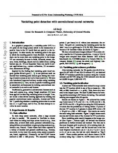
We evaluated our CNN architecture on the normalized-uniform NORB dataset [4], consisting of each 24,300 binocular grayscale training and testing images. After training on the raw pixel data for 360 epochs (equal to 291,000 mini-batch updates), an error rate of 8.6% on the test set was achieved. The speed of our implementation was benchmarked on a system with an Intel Core i7 940 (2.93 GHz) CPU and a GeForce GTX 285. For a comparison of the runtime we implemented an equivalent single-threaded, sequential CPU version which was optimized for speed by the compiler. The most critical components of the parallel implementation are the forward pass and the backpropagation of error. For both, several patterns are processed in parallel, and it is to be expected that a larger speedup 3

Speedup compared to CPU

120 100 80 60 40 20

Forward propagation Backpropagation

0 0

30

60 90 Number of patterns

120

150

Figure 5: Speedup factor of the GPU implementation for the number of patterns trained in parallel (compared to a serial CPU version).

Figure 6: Two desktop supercomputers, each consisting of eight GPUs, for a total of 3840 multiprocessor cores.

can be achieved for an increasing number of patterns. As shown in Figure 5, the highest speedup was achieved when the number of patterns is a multiple of 30, because the GTX 285 consists of 30 multiprocessors. If more then 30 patterns are scheduled, the remaining patterns are queued until another multiprocessor has finished. One of the largest networks tested consists of four 512×512 pixel input maps and 8, 32, 64 and 64 feature maps on the successive convolutional layers, followed by two fully-connected layers with 100 and 10 neurons, respectively. One training pass (including all memory transactions) required 34.1 ms per pattern on GPU, compared to 3751.8 ms on CPU. We found that data transfer times are negligible compared to forward and backward propagation. From further benchmarks with various reasonably sized networks we can deduce that neither network size, nor the size of the input has a significant influence on the speedup of our implementation. In all cases, the gradient descent mini-batch learning was accelerated by a factor ranging from 95 to 115.

6 Conclusions Our work shows that current graphics cards programming frameworks with their hierarchy of threads are very well suited for a parallel implementation of CNNs. In comparison to a serial CPU implementation we were able to significantly speed up the learning algorithm by a factor ranging from 95 to 115 on a single GPU. Until now it was impossible to study deep CNNs with high-resolution input images due to the tremendous computational power required for their training. The aim for our future work is to extend this approach to systems with multiple GPUs (shown in Figure 6) and to apply such large-scale CNNs to pattern recognition tasks using datasets with high-resolution natural images.

References [1] S. Behnke. Hierarchical Neural Networks for Image Interpretation, volume 2766 of Lecture Notes in Computer Science. Springer-Verlag New York, Inc., Secaucus, NJ, USA, 2003. [2] H. Larochelle, Y. Bengio, J. Louradour, and P. Lamblin. Exploring Strategies for Training Deep Neural Networks. The Journal of Machine Learning Research, pages 1–40, 2009. [3] Y. LeCun, L. Bottou, Y. Bengio, and P. Haffner. Gradient-Based Learning Applied to Document Recognition. Proceedings of the IEEE, 86(11):2278–2324, 1998. [4] Y. LeCun, F. Huang, and L. Bottou. Learning Methods for Generic Object Recognition with Invariance to Pose and Lighting. In Proceedings of CVPR’04. IEEE Press, 2004. [5] Nvidia Corporation. CUDA Programming Guide 2.2, Apr. 2009. [6] M. Osadchy, Y. LeCun, and M. Miller. Synergistic Face Detection and Pose Estimation with Energy-Based Models. Journal of Machine Learning Research, 8:1197–1215, 2007. [7] M. Riedmiller and H. Braun. RPROP – A fast adaptive learning algorithm. In Proceedings of the Int. Symposium on Computer and Information Science VII, 1992. [8] P. Y. Simard, D. Steinkraus, and J. C. Platt. Best Practice for Convolutional Neural Networks Applied to Visual Document Analysis. In ICDAR, IEEE, Los Alamitos, pages 958–962, 2003.

4