NAS Technical Report NAS-09-003, November 2009
Acceleration of a CFD Code with a GPU Dennis C. Jespersen
ABSTRACT The Computational Fluid Dynamics code Overflow includes as one of its solver options an algorithm which is a fairly small piece of code but which accounts for a significant portion of the total computational time. This paper studies some of the issues in accelerating the code by using a Graphics Processing Unit (GPU). The algorithm needs to be modified to be suitable for a GPU, and attention needs to be given to 64-bit and 32-bit arithmetic. Interestingly, the work done for the GPU produced ideas for accelerating the CPU code and led to significant speedup on the CPU. Keywords: GPU, acceleration, Overflow code 1. INTRODUCTION Computational Fluid Dynamics (CFD) has a history of seeking and requiring ever higher computational performance. This quest has in the past been satisfied mainly by faster clock speeds. The era of increasing clock rates has reached a plateau, due mainly to heat dissipation constraints. A boost in computational performance without increasing clock speed can be supplied by parallelism. This parallelism can come in the form of task parallelism, data parallelism, or perhaps a combination of the two. Common current paradigms for implementing parallelism are explicit message-passing with MPI [12] for either distributed or shared memory systems and OpenMP [13] for shared memory systems. A hybrid paradigm is also possible, with OpenMP on multiprocessor nodes and MPI among the nodes. A Graphics Processing Unit (GPU) is a processor specialized for graphics rendering. Much work has recently been focused on GPUs as devices that can be used in general-purpose computing. A GPU can produce a very high Flop/s (floating-point operations per second) rate if an algorithm is well-suited for the device. There have been several studies illustrating the acceleration of scientific computing codes that is possible by using GPUs [2, 6, 10]. In this paper we study the issues in accelerating a well-known CFD code, Overflow, on a GPU. Dennis Jespersen, MS 258-2, NASA/Ames Research Center, Moffett Field, CA 94035, U.S.A.,
[email protected].
1
NAS Technical Report NAS-09-003, November 2009
2. OVERFLOW CODE The Overflow code [3, 4, 5, 9] is intended for the solution of the Reynoldsaveraged Navier-Stokes equations with complex geometries. The code uses finite differences on logically Cartesian meshes. The meshes are body-fitted and geometric complexity is handled by allowing the meshes to arbitrarily overlap one another. Overflow uses implicit time-stepping and can be run in time-accurate or in steady-state modes. Implicit time-stepping is used because implicit methods tend to mitigate severe stability limits on the size of the time step that arise for explicit methods on highly-stretched grids that are common for viscous flow problems at high Reynolds numbers. A consequence of implicit time-stepping is that some method is needed to approximately solve the large system of equations that arises when stepping from one time level to the next. The Overflow user needs to specify physical flow inputs, such as Mach number and Reynolds number, and boundary conditions which typically define solid walls and inflow or outflow regions. Along with these physics-type inputs there are inputs which choose particular numerical algorithms and specify parameters for them. The basic equation of fluid motion solved by Overflow is of the form Qt + L(Q) = f (Q),
(1)
where Q is the vector of flow variables, L(Q) denotes all the spatial differencing terms, and f (Q) denotes terms from boundary conditions and possible source terms. The basic equation (1) is written in “delta form” [1, 8] A(∆Qn+1 ) = Rn ,
(2)
where A is a large sparse matrix which is not explicitly constructed, ∆Qn+1 = Qn+1 − Qn , and Rn involves the discretization of the L(Q) terms at time level n. The user of Overflow must choose among several possible discretizations (e.g. central differencing, Total Variation Diminishing, Roe upwind). Each of these choices typically requires further user specification of numerical parameters, e.g. dissipation parameters or type of flux limiter and parameters for the limiter. Finally the user needs to decide which implicit algorithm to use: some choices are factored block tridiagonal, factored scalar pentadiagonal, LU-SGS. Over the years the code evolved and expanded to incorporate six basic choices for the implicit part of the algorithm. 3. GPU CONSIDERATIONS GPU cards were originally hard to program and had a steep learning curve. The advent of less daunting interfaces such as CUDA [11] has led to an explosion of interest in using GPUs for numerically intensive work in scientific computing. For our purposes here the key issues of GPU cards are massive parallelism (hundreds or thousands of threads), mostly SIMD parallelism, 32-bit floating point arithmetic, and the overhead of data traffic between the CPU and GPU. For a GPU to successfully accelerate a piece of code the code must be amenable to large-scale SIMD parallelism, must tolerate 32-bit floating-point arithmetic,
2
NAS Technical Report NAS-09-003, November 2009
and must contain enough computational work to amortize the cost of transferring data from the CPU to the GPU and transferring results back from the GPU to the CPU. (Recent GPU hardware supports some limited 64-bit arithmetic but 32-bit arithmetic is significantly faster.) We will see that the SSOR algorithm in Overflow is not well-suited to a GPU, but that a Jacobi version of the algorithm might be suitable for a GPU. 4. THE SSOR ALGORITHM IN OVERFLOW In an attempt to ease the user’s burdensome task of selecting algorithm options and choosing parameters which may change for each class of flow problem, recently another option was added for the implicit part of Overflow with the hope that it would be widely applicable and would be almost universally usable [7]. This algorithm is called in the references an SSOR algorithm, but it is strictly speaking a mix of an SSOR algorithm and a Jacobi algorithm, a “quasi-SSOR” algorithm. The key step of the quasi-SSOR algorithm is as follows. At each grid n point with index (j, k, l) one computes a residual Rjkl and 5 × 5 matrices AJ, AK, AL, CJ, CK, CL; these matrices depend on the flow variables at the neighboring grid points, and are fixed during the SSOR iterations. Then, with iteration stage denoted by a superscript n and with a relaxation parameter ω, relaxation steps are of the form ∆Qn+1 = (1 − ω)∆Qnjkl jkl n+1 n +ω(Rjkl − AJjkl ∆Qnj−1,k,l − AKjkl ∆Qn+1 j,k−1,l − ALjkl ∆Qj,k,l−1 −CJjkl ∆Qnj+1,k,l − CKjkl ∆Qnj,k+1,l − CLjkl ∆Qnj,k,l+1 ) (3) n+1 for a forward sweep (assuming the 5-vectors ∆Qn+1 j,k−1,l and ∆Qj,k,l−1 have been computed, and updating all ∆Qjkl as soon as a full line of j values has been computed), and a step of the form
∆Qn+1 = (1 − ω)∆Qnjkl jkl n +ω(Rjkl − AJjkl ∆Qnj−1,k,l − AKjkl ∆Qnj,k−1,l − ALjkl ∆Qnj,k,l−1 n+1 −CJjkl ∆Qnj+1,k,l − CKjkl ∆Qn+1 j,k+1,l − CLjkl ∆Qj,k,l+1 )
(4)
n+1 for a backward sweep (again assuming ∆Qn+1 j,k+1,l and ∆Qj,k,l+1 have been computed). The forward/backward pair is then iterated. This algorithm is not strictly speaking an SSOR algorithm; it is Jacobi in j-lines and SSOR in k-l planes. We will refer to it as SSOR for simplicity. This algorithm needs the 6 nearest spatial neighbors of ∆Qnjkl , some at iteration level n and some at iteration level n + 1. The SSOR algorithm is a modest-sized subroutine but it may consume 80% of the total runtime of the code, so it is a computational hot spot. The modest size of the subroutine and the large fraction of total time consumed by the algorithm make using a GPU as a coprocessor to accelerate the code an attractive idea. Unfortunately, the algorithm as it stands is not suited to a GPU due to the dependencies of the iteration, namely ∆Qn+1 appears on the right-hand side of equations (3) and (4). An algorithm that would be suited to a GPU would be
3
NAS Technical Report NAS-09-003, November 2009
a Jacobi algorithm with relaxation steps of the form ∆Qn+1 = (1 − ω)∆Qnjkl jkl n +ω(Rjkl − AJjkl ∆Qnj−1,k,l − AKjkl ∆Qnj,k−1,l − ALjkl ∆Qnj,k,l−1 −CJjkl ∆Qnj+1,k,l − CKjkl ∆Qnj,k+1,l − CLjkl ∆Qnj,k,l+1 ) (5) Here we could envision assigning a thread of computation to each grid point and the threads could compute independently of one another because there are no ∆Qn+1 terms on the right-hand side of (5). It is important to realize that the Jacobi algorithm might be less robust or might converge slower than the original SSOR algorithm. Fully discussing this would take us too far afield, though we will show some convergence comparisons of Jacobi and SSOR. The work presented here proceeded in several stages: 1. Implement a Jacobi algorithm on the CPU using 64-bit arithmetic; compare performance and convergence/stability of Jacobi and SSOR. 2. Implement a Jacobi algorithm on the CPU using 32-bit arithmetic; compare performance and convergence/stability of 64-bit and 32-bit Jacobi. 3. Implement a Jacobi algorithm on the GPU; compare performance of the GPU algorithm with the 32-bit CPU algorithm. 5. IMPLEMENTATION AND RESULTS The first stage of the work, implementing the Jacobi algorithm on the CPU using 64-bit arithmetic, was straightforward. We compare in Figure 1 convergence for the SSOR and Jacobi algorithms on two test cases. The first test case is turbulent flow over a flat plate with a 121 × 41 × 81 grid. The second flow is turbulent flow in a duct with a 166 × 31 × 49 grid. Both cases show, unsurprisingly, that asymptotic convergence of the Jacobi algorithm is slightly slower than that of the SSOR algorithm. Both cases reach machine zero (solution converged to 64-bit accuracy). The SSOR algorithm is slightly faster in terms of wallclock seconds per time step, because the SSOR algorithm updates ∆Q as the computation proceeds whereas the Jacobi algorithm uses an extra three-dimensional array to store the changes to ∆Q and then sweeps through the full ∆Q array to form the new values of ∆Q. Implementing the Jacobi algorithm in 32-bit arithmetic for the CPU was tedious but straightforward. The implementation included making 32-bit versions of all the subroutines dealing with the computation of the left-hand side matrices (about 50 subroutines) and copying, on the front-end, the flow variables and metric terms to 32-bit quantities; in all, 28 words per grid point were copied from 64-bit to 32-bit representation. In Figure 2 we show convergence for the Jacobi algorithm in 64-bit arithmetic and in 32-bit arithmetic for the two test cases. To plotting accuracy there is no difference in convergence between the 32-bit and 64-bit Jacobi algorithms. This verifies for these cases that full 64-bit solution accuracy can be obtained with a 32-bit Jacobi algorithm. Finally the Jacobi algorithm was implemented on the GPU. The strategy was to compute all the matrices AJ, etc., on the CPU and transfer them to the GPU. The Jacobi algorithm itself, just one subroutine, was hand-translated into CUDA code. This strategy avoided a long error-prone translation of many
4
NAS Technical Report NAS-09-003, November 2009
Turbulent flat plate
-7
10
-8
-8
10
SSOR, 64-bit Jacobi, 64-bit
-9
10
-10
10
-9
10
-10
10
10
-11
-11
10
10
-12
L2 residual
3D Duct
-7
10
-12
10
10
-13
-13
10
10
-14
-14
10
10
-15
-15
10
10
-16
-16
10
10
-17
-17
10
10
-18
-18
10
10
-19
-19
10
10 0
5000
10000 15000 Time step
20000
0
10000
20000 Time step
30000
40000
Figure 1. SSOR and Jacobi convergence, 64-bit arithmetic
Fortran subroutines into CUDA, but this strategy may be suboptimal as the matrices themselves could be computed on the GPU. We found no difference between convergence of the 32-bit Jacobi algorithm on the CPU and on the GPU, so the slight differences in details of floating-point arithmetic between the CPU and the GPU have no impact for these cases. Now we consider performance of the code. The metric we use is wallclock seconds per step, so lower is better. The GPU algorithm was coded in several slightly different ways, varying in the way the data were laid out on the GPU and whether or not shared memory on the GPU was used. Data shown are for the best-performing GPU variant. The work here was done on two platforms. The first platform was a workstation equipped with a 2.1 GHz quad-core AMD Opteron 2352 processor. The host compiler system was the Portland Group compiler suite version 8. The TABLE I. Implicit solver times, sec/step (lower is better)
Algorithm SSOR CPU Jacobi GPU GPU/CPU
G machine T machine Plate Duct Plate Duct 3.51 2.14 3.83 2.33 1.43 0.91 1.35 0.76 0.41 0.43 0.35 0.33
5
NAS Technical Report NAS-09-003, November 2009
Turbulent flat plate
-7
10
-8
-8
10
Jacobi, 64-bit Jacobi, 32-bit
-9
10
-10
10
-9
10
-10
10
10
-11
-11
10
10
-12
L2 residual
3D Duct
-7
10
-12
10
10
-13
-13
10
10
-14
-14
10
10
-15
-15
10
10
-16
-16
10
10
-17
-17
10
10
-18
-18
10
10
-19
-19
10
10 0
5000
10000 15000 Time step
20000
0
10000
20000 Time step
30000
40000
Figure 2. Jacobi convergence, 64-bit and 32-bit arithmetic
GPU card was a 1.35 GHz NVIDIA GeForce 8800 GTX with 128 cores and 768 MB of global memory. The connection between CPU and GPU was a PCI Express 16X bus. The programming interface was CUDA version 1.0. This platform will be referred to as the “G machine.” The second platform was a workstation equipped with two 2.8 GHz dualcore AMD Opteron 2220 processors. The GPU card was a 1.30 GHz NVIDIA Tesla C1060 with 240 cores and 4 GB of global memory. For this machine, the source code was cross-compiled on the first machine using the Portland Group compiler. This platform will be referred to as the “T machine.” Tables I and II give performance data for the two test cases on the two machines. The implicit solver times in Table I (which include a small amount of work on the CPU as well as the actual relaxation algorithm) show a speedup on the GPU by about a factor of between 2.5 and 3. The reason the T machine TABLE II. Total time for CPU and GPU, sec/step (lower is better)
Algorithm SSOR CPU Jacobi GPU GPU/CPU
G machine T machine Plate Duct Plate Duct 6.96 4.21 7.93 4.85 4.41 2.66 5.04 3.12 0.63 0.63 0.64 0.64
6
NAS Technical Report NAS-09-003, November 2009
TABLE III. GPU Kernel times, sec/step (lower is better)
GPU total GPU kernel only
GTX8800 Tesla C1060 Plate Duct Plate Duct 0.904 0.576 0.314 0.193 0.784 0.499 0.142 0.082
TABLE IV. SSOR performance on CPU, 64-bit and 32-bit (sec/step)
G machine T machine Algorithm Plate Duct Plate Duct SSOR-64 CPU 6.96 4.21 7.93 4.85 SSOR-32 CPU 5.55 3.34 6.30 3.87 SSOR-32/SSOR-64 0.80 0.79 0.79 0.80
times are only slightly better than the G machine times is that the times shown here include some CPU work, and for some unknown reason the CPU routines involved ran faster on the G machine than on the T machine. The total wallclock time, which is the quantity of ultimate interest to the code user, decreases by about 40%, as seen in Table II. Again, the G machine is overall faster than the machine with the T machine, because the parts of the code that execute on the CPU are for some reason faster on the G machine. Table III gives GPU total time (kernel plus time for data transfer) and GPU kernel time for these cases. For the GTX8800 device, the kernel which gave the best overall code performance was a kernel which mapped each grid point to a different thread on the GPU (thanks to Jonathan Cohen of NVIDIA for showing a nice way to do this) and which used some shared memory. For the Tesla device, the kernel which gave the best overall code performance was a kernel involving a two-dimensional mapping of the first two grid dimensions onto the device, a loop in the 3rd dimension, and 16 threads per grid point with the 5 × 5 matrices on the CPU stored in an array of size 32. For both the Tesla and the GTX8800 devices there are data layouts which give better performance of the GPU considered in isolation, but these layouts involve data motion on the CPU and this data motion loses more wallclock time than is gained by the faster kernel. 6. IMPACT OF GPU WORK ON CPU CODE These results are encouraging. It seems that the Jacobi GPU algorithm is significantly faster than the SSOR CPU algorithm, since Table II shows a speedup for the whole code of about 40%. This is a significant speedup considering that the only code being executed on the GPU is a small piece of the implicit side, and there are no changes to the flow explicit side or to the turbulence model. However, further reflection indicates that more performance can be gained from the CPU. Specifically, the SSOR CPU algorithm could be changed to use 32-bit arithmetic. Experience has shown that Overflow is a cache and bandwidth-limited code, so use of 32-bit arithmetic (where applicable) should
7
NAS Technical Report NAS-09-003, November 2009
TABLE V. SSOR and OpenMP performance on CPU (sec/step)
Algorithm SSOR-64 SSOR-64 SSOR-64 Revised SSOR-64 Revised SSOR-64 Revised SSOR-64 SSOR-32 SSOR-32 SSOR-32 Revised SSOR-32 Revised SSOR-32 Revised SSOR-32
OpenMP threads 1 2 4 1 2 4 1 2 4 1 2 4
G machine T machine Plate Duct Plate Duct 6.96 4.21 7.93 4.85 5.53 3.27 6.76 4.11 4.60 2.80 5.94 3.60 7.79 4.70 8.41 5.14 4.79 2.85 4.76 2.96 3.36 2.04 3.27 1.99 5.55 3.34 6.30 3.87 4.23 2.55 4.72 2.89 3.45 2.11 3.92 2.41 6.07 3.65 6.92 4.20 3.63 2.18 3.79 2.37 2.38 1.47 2.50 1.52
significantly speed up the code due to the effective doubling of cache size and bandwidth. This motivated the implementation of a 32-bit SSOR algorithm on the CPU. Convergence for this algorithm, for the plate and duct test cases, was identical to convergence for the 64-bit SSOR algorithm. Single-core performance for the 32-bit SSOR algorithm is compared with performance for the 64-bit SSOR algorithm in Table IV. Total wallclock time is reduced by 20% by the use of 32-bit arithmetic; this is a significant speedup for such an unsophisticated code modification. Even more performance can be gained on the CPU by taking advantage of the multiple cores found in essentially all contemporary scientific computing environments. Overflow has long had OpenMP capability, but the SSOR algorithm as originally coded in Overflow was not amenable to OpenMP parallellism (as mentioned in section 4, the original coding was Jacobi in the j index and Gauss-Seidel in the k and l indices, while the OpenMP parallelism in Overflow is parallelism in l). Revising the algorithm to be Jacobi in l and Gauss-Seidel in j and k allowed the use of OpenMP for the SSOR algorithm. The revised SSOR algorithm had the same convergence characteristics as the Jacobi algorithm for the duct and plate test cases. The revised algorithm can also be coded in 64-bit or 32-bit arithmetic. We show in Table V performance for these algorithms and various numbers of OpenMP threads; these are all CPU performance numbers, the GPU is not involved here, and this is performance for the full code. For a single OpenMP thread the revised SSOR algorithm is slower than the original, due to poorer cache utilization, but for 2 or 4 OpenMP threads the revised algorithm is faster than the original. Finally, Table VI gives performance data for the two platforms using the Jacobi algorithm on the GPU and OpenMP threads on the CPU. To compare the code with and without GPU but otherwise using all the computational resources, the best numbers in Table V should be compared with the best numbers in Table VI. The result is that for the workstation with the GTX8800 GPU, the
8
NAS Technical Report NAS-09-003, November 2009
TABLE VI. Jacobi on GPU + OpenMP on CPU, performance (sec/step)
OpenMP threads on CPU 1 2 4
GTX8800 Tesla C1060 Plate Duct Plate Duct 4.39 2.66 4.58 2.85 3.10 1.78 2.92 1.83 2.32 1.42 1.90 1.18
best time with GPU is just a few percent faster than the best time without GPU, whereas for the workstation with the Tesla C1060 GPU, the best time with GPU is about 25% better than the best time without GPU. (The ultimate reason for the better performance of the Tesla C1060 on this code is the relaxed alignment restrictions for coalesced loads as compared to the GTX8800.) Even this is not the end of the story, as there are further opportunities for moving computation from the CPU to the GPU. For example, the matrices can be computed in parallel, so this part of the computation, which is now executed by the CPU, can be moved to the GPU. These and other optimizations are currently under investigation. 7. CONCLUSIONS The work presented in this paper has shown a speedup by a factor of between 2.5 and 3 for the SSOR solver in Overflow and a total wallclock time decrease of about 40%, for a GPU as compared to a single CPU. The GPU work gave ideas and motivation for accelerating the code on multi-core CPUs, so that currently the CPU+GPU code is about 25% faster than the pure CPU code. This study has until now focused on obtaining improved performance with a one CPU + one GPU combination. This is the first step to enhancing Overflow performance via GPUs on realistic problems. However, for almost all realistic cases, Overflow is used with MPI (Message-Passing Interface) and many CPUs. The work here extends naturally to any cluster with a number of multi-core nodes, each node also containing a GPU. Overflow could be used in hybrid mode, with each node corresponding to an MPI process, and each MPI process would have multiple OpenMP threads. The hyperwall-2 at NASA/Ames Research Center [14] is such a cluster and the version of Overflow with GPU capability has run on the hyperwall-2 as a proof of concept. It is worthwhile to note that the work done here has affected the Overflow code. The latest official release (version 2.1ac) of Overflow has completely abandoned the 64-bit version of the SSOR algorithm in favor of the 32-bit version, and the revised SSOR algorithm (32-bit arithmetic only) is available as an option. The speedups due to 32-bit arithmetic were so compelling that 64-bit arithmetic is no longer even an option in these portions of the code. This may give food for thought when considering the need for 64-bit arithmetic on GPUs.
9
NAS Technical Report NAS-09-003, November 2009
ACKNOWLEDGMENTS This work was partially supported by the Fundamental Aeronautics program of NASA’s Aeronautics Research Mission Directorate. NVIDIA Corporation donated the Tesla C1060 hardware. REFERENCES 1. Beam, R., and Warming, R.F. 1976. “An Implicit Finite-difference Algorithm for Hyperbolic Systems in Conservation Law Form.” J. Comp. Physics, 22(1):87-110. 2. Brandvik, T., and Pullan, G. 2008. “Acceleration of a 3D Euler Solver Using Commodity Graphics Hardware,” AIAA 46th Aerospace Sciences Meeting, Reno, NV, paper no. AIAA2008-607. 3. Buning, P. G., Chiu. I. T., Obayashi, S., Rizk, Y. M., and Steger, J. L. 1988. “Numerical Simulation of the Integrated Space Shuttle Vehicle in Ascent,” AIAA Atmospheric Flight Mechanics Conference, paper no. 88-4359-CP. 4. Kandula, M. and Buning, P. G. 1994. “Implementation of LU-SGS Algorithm and Roe Upwinding Scheme in OVERFLOW Thin-layer Navier-Stokes Code,” AIAA 25th Fluid Dynamics Conference, Colorado Springs, CO, paper no. AIAA-94-2357. 5. Meakin, R. L. 2001. “Automatic Off-body Grid Generation for Domains of Arbitrary Size,” AIAA 15th Computational Fluid Dynamics Conference, Anaheim, CA, paper no. AIAA2001-2536. 6. Michalakes, J. and Vachharajani, M. 2008. “GPU Acceleration of Numerical Weather Prediction,” Parallel Processing Letters, 18(4):531-548. 7. Nichols, R. H., Tramel, R. W., and Buning, P. G. 2006. “Solver and Turbulence Model Upgrades to OVERFLOW 2 for Unsteady and High-speed Applications,” AIAA 24th Applied Aerodynamics Conference, San Francisco, CA, paper no. AIAA-2006-2824. 8. Pulliam, T. H. and Chaussee, D. S. 1981. “A Diagonalized Form of an Implicit Approximate Factorization Algorithm,” J. Comp. Phys., 39(2):347-363. 9. Renze, K. J., Buning, P. G., and Rajagopalan, R. G. 1992. “A Comparative Study of Turbulence Models for Overset Grids,” AIAA 30th Aerospace Sciences Meeting, Reno, NV, paper no. AIAA-92-0437. 10. Thibault, J. C. and Senocak, I. 2009. “CUDA Implementation of a Navier-Stokes Solver on Multi-GPU Desktop Platforms for Incompressible Flows,” AIAA 47th Aerospace Sciences Meeting, Orlando, FL, paper no. AIAA-2009-758. 11. http://www.nvidia.com/object/cuda home.html. 12. http://www-unix.mcs.anl.gov/mpi. 13. http://www.openmp.org. 14. http://www.nas.nasa.gov/News/Releases/2008/06-25-08.html.
10