Systematic Sampling and Cluster Sampling of Packet Delays Thomas Lindh Laboratory for Communication Networks, LCN School of Electrical Engineering Royal Institute of Technology, KTH
[email protected]
Abstract. Based on experiences of a traffic flow performance meter this paper suggests and evaluates cluster sampling and systematic sampling as methods to estimate average packet delays. Systematic sampling facilitates for example time analysis, frequency analysis and jitter measurements. Cluster sampling with repeated trains of periodically spaced sampling units separated by random starting periods, and systematic sampling are evaluated with respect to accuracy and precision. Packet delay traces have been used in simulation studies. The motivation for this kind of cluster sampling is to avoid performance deterioration due to possible periodic patterns in packet delays. The conclusion of this study is that systematic sampling and cluster sampling methods are efficient alternatives, or complements, to simple random sampling.
1 Introduction This paper derives from two sources. One origin is the results and experiences of a measurement method implemented as an extension to the traffic flow meter NeTraMet ([1], [2] and [3]). The method uses monitoring packets for collecting samples of packet delays. The second motivation is to present and evaluate an alternative to the often recommended method based on simple random sampling (or Poisson sampling). The paper focuses on packet delay estimates and is structured in the following way. Section 2 gives a brief background to the problem and our hypotheses. The main characteristics of cluster sampling, systematic sampling and metrics for performance comparison are summarized in Section 3 and Section 4. Results from simulations based on actual packet delay traces are found in Section 5 and Section 6. The two concluding sections contain a discussion of the results and the main conclusions. Tables and figures from performance evaluation based on delay traces are found in the Appendix.
2 Sampling Issues and Hypotheses Poisson sampling, or simple random sampling, is often a recommended method based on statistical considerations [4]. The main argument is that periodic sampling might produce biased and imprecise results if the sampling process coincides with periodic patterns in the data traffic. The PASTA principle (Poisson arrivals see time averages) is often referred to as the theoretical basis for the superiority of Poisson sampling in comparison to e.g. systematic sampling. However, periodic streams of sampling units are advantageous for presentation and analysis of time series and spectral properties. Periodic sampling is suggested as an alternative in e.g. RFC 3432 (Network performance measurements with periodic streams). As argued in this RFC, periodic sampling is particularly well suited for multimedia and voice applications. Periodic sampling also facilitates one-point jitter measurements. Some studies also indicate that Poisson sampling and periodic sampling do not show significantly different performance results in estimating packet delays ([5], [6] and [13]). Low frequency components have been found in network delays with time scales that not seem relevant packet delay sampling methods [7]. Cluster sampling is here defined as periods of systematic sampling interrupted by silent periods of random length, i.e. trains of periodic sampling separated by random starting periods (Figure 1). This paper proposes an alternative, or complement, to sampling of network performance parameters. The hypotheses discussed in the remainder of the paper are the following. ♦ ♦
In traffic cases with low auto-correlation, systematic sampling with random start is at least as effective as simple random sampling. In traffic cases with considerable auto-correlation and periodic patterns, cluster sampling is an alternative with a level of efficiency that is comparable to simple random sampling.
Fig. 1. The primary units in cluster sampling consist of trains of secondary units with constant intervals between the sampled packets. The trains are separated by starting periods of random length (dotted lines in the figure).
3 Systematic Sampling and Cluster Sampling Sampling methods are described in a number of textbooks. The survey in this section is based on Cochran [8], Thompson [9], Murthy [10], Sukhatme [11] and Raj [12]. In simple random sampling (SRS) the sampled units are chosen randomly from
a population where all units should have equal probability to be selected. Systematic sampling and cluster sampling are described below. 3.1 Systematic Sampling In systematic sampling with random start the first sampled unit is chosen randomly from the first k units in a population. The remainder of the sampling units in the sample consists of every kth element in the population. Systematic sampling, often called periodic sampling in data communication, can be seen as a special case of cluster sampling, where a number of primary units are chosen randomly from a population. The primary units (clusters) consist of secondary units (subunits), which contain the actual sampled entities. In systematic sampling a single primary unit consists of secondary units spaced in some systematic fashion throughout the population [9]. Having chosen a primary unit randomly among the first k elements in a population, then all secondary units are determined, each separated by an equal distance k. An advantage of systematic sampling is that the sampling units are evenly spread over the entire population. However, this sampling scheme is sensitive to correlation between units in the population. A positive auto-correlation decreases the precision while a negative auto-correlation will improve the precision compared to simple random sampling. 3.2 Cluster Sampling In cluster sampling, several primary units are chosen randomly, each with the secondary units that contain the sampling units. The method implements repeated sequences of trains, where each train contains periodically spaced sampling units proceeded by a starting phase of random length (Figure 1). In a way this is similar to a stratified sampling scheme, where each stratum consists of a random starting phase followed by periodic sampling units. A motivation for applying cluster sampling is that systematic sampling is not robust against periodic patterns and high auto-correlation. Systematic sampling begins with a random starting period, but thereafter the intervals between the following sampled units are predetermined. Trains of systematically sampled units, each separated by a random starting period, are more appropriate under such conditions. Assume that a sampled entity is picked every kth packet on average. If pulses (consisting of s packets) are repeated periodically in the population with an interval of k packets, then the probability to choose a packet from exactly those pulses will be s⎞ ⎛s⎞ ⎛ ⎜ ⎟ , and the probability to avoid this pulse ⎜1 − ⎟ . If n number of trains are used, ⎝ k⎠ ⎝k⎠ each with a random starting interval, then the probability that all trains coincide with n
⎛s⎞ the periodic pulses is ⎜ ⎟ , and the probability that no train coincides with the peri⎝k⎠
n
⎛ s⎞ odic pulses is ⎜1 − ⎟ . The probability that at least one train coincides with the ⎝ k⎠ n
⎛ s⎞ periodic pattern is 1 − ⎜1 − ⎟ . ⎝ k⎠ As n grows, the probability that the samples will coincide completely with (or completely avoid) a periodic pattern will decrease. This means that repeated trains with systematic sampling and random starting intervals are better suited to prevent imprecise results due to impact of periodic patterns.
4 Performance Comparison of Sampling Methods The following metrics and equations are used to evaluate the precision and accuracy of sampling methods ([8], [9], [10], [11] and [12]). The relative error of an estimator is given by ˆ −Θ Θ E= , (1) Θ ˆ is the estimate of the parameter. where Θ is the parameter in the population, and Θ m−M For a mean value estimator Equation (1) will be, E = , where M is the popuM lation mean value and m is the estimate based on the sample mean value. The variance of the mean value simple random estimator , y srs , is N −n S2 (2) ⋅ , N n where N is the total population, n is the number of sampling units, and S2 is the variance of the population, which can be estimated as the sample variance, s2. The standard error of a mean value estimator , y , is given by V ( y srs ) =
S
, (3) n where S is the standard deviation of the population, which can be estimated as the sample standard deviation, s. The variance of a mean value estimator using systematic sampling , ysy , is σy =
2 V ( ysy ) = S 2 − Swsy ,
(4)
where S is the standard deviation of the population and Swsy is the standard deviation of the samples (within systematic samples), which can be estimated from the samples (s and swsy). Intuitively it is obvious that the sample should be heterogeneous and have a relatively high variance in order to give a good representation of the population. The variance of the mean value estimate in systematic sampling depends on the degree of correlation in delay data. This can be expressed as
N −1 S2 (5) [1 + (n − 1) ρ ] , ⋅ N n where ρ is the coefficient of correlation within samples with lag one (between pairs of sampling units). A negative correlation coefficient reduces the variance. If ρ is upwards concave it complies with the condition ρ u ≥ ρ v , u < v , and that ρ u +1 + ρ u −1 − 2 ρ u ≥ 0 , where u and v are distances between sampling units. In this case systematic sampling is more effective than stratified sampling, which in turn is more efficient than simple random sampling ([8] and [9]). The variance of an estimator based on cluster sampling , ycluster , is given by V ( y sy ) =
1− f S 2 [1 + (M − 1) ρ ] , f = n . ⋅ (6) N M n Randomly, n clusters (primary units) are chosen among N possible clusters. Each of these primary units consists of M secondary units, and ρ is the correlation coefficient between the primary units (intra-cluster) [8]. The relative error measures possible bias, and the ratio between the standard error for systematic (or cluster) sampling and SRS is a measure of the relative precision of the estimates. V ( ycluster ) =
5 Simulation and Evaluation Procedure Packet delay traces from several different sources have been used to evaluate systematic sampling with random start, cluster sampling with trains of periodic sampling units separated by random starting intervals, and simple random sampling. A MATLAB simulation program computes the relative error, the standard error and the correlation coefficient based on delay packet data. These delay traces represent oneway delays in the core of an operator’s network and round-trip times in access networks. Periodic pulses are added to the delay traces in order to raise the correlation, and the same measures as above are computed in these cases. The amplitude of each added pulse is equal to one half of the maximum delay. The distance between these periodic pulses is the same as the distance between the sampling units in systematic and cluster sampling (and the average distance between sampling units for simple random sampling). The purpose is to arrange a worst case scenario for systematic sampling. The results from two of the case studies are presented in the paper; one-way delays in the core of an operator’s network, and round-trip times between a client in a residential access network and a server at KTH. Table I (Appendix) contains results from delays in an operator’s network In Table II auto-correlation deliberately has been increased by adding periodic pulses. Table III shows the results for the round-trip delays between a client in an access network and a server. The tables in Appendix contain the following information. ♦
The size of the monitoring block and the corresponding sample size (the number of sampled units) in the first two columns.
♦ ♦ ♦ ♦ ♦
The number of trains in cluster sampling in column three. The average relative errors in estimating the mean value for systematic/cluster sampling and simple random sampling in the forth and the fifth columns. The average measured standard errors in estimating the mean value for systematic (cluster) sampling and simple random sampling in the sixth and the seventh columns. The average ratio between the standard error using systematic (cluster) sampling and SRS in the eighth column. The average correlation coefficients between pairs of units in the samples (i.e. with lag one) for systematic (cluster) sampling (ρsy) and SRS (ρsrs) in column nine and column ten. The correlation coefficient for the entire population (packet delay trace) with a lag equal to the distance between the sampled units in systematic or cluster sampling in the eleventh column.
6 Performance Results The relative error, which indicates possible bias in estimating the mean delay, is below 10-3 in all traces (with samples of 100 or more units). Periodically inserted pulses will increase the relative errors, however seldom above 10-2. No significant difference between the sampling methods can be noticed in these cases. The standard error is a measure of a sampling method’s precision. As expected, the measured standard error (the standard deviation of the sample means) is reduced as the number of sampling units increases (Table I). This agrees with Equation (3). In Table I the standard error ratio between systematic sampling (one train) and SRS, is approximately equal to 1 in the majority of tests, and falls below 1 when cluster sampling is applied. For the highest ratio (R=1.33) in Table I, the statistical uncertainty will be as follows. For a confidence level of 95%, the SRS estimator gives a confidence half interval of 3.2 µs, and for the systematic estimator the half interval is 2.4 µs. The mean value is 15.48 ms, which means that the difference in precision is marginal. The correlation coefficient between pairs of units in the samples stretches from − 0.04 to 0.05. No significant difference for the sampling methods can be seen. If a periodic pattern is added to the delay traces (Table II), the standard error ratio increases considerably (the ratio stretches from 5 to 25 for systematic sampling compared to SRS). The distance between the inserted pulses is the same as between the periodic sampling units. As can be seen in Table II, the correlation coefficient for the population with a lag equal to the distance between the inserted pulses, is approximately 1 (one). This ratio decreases if several trains are used. A ratio between 2 and 4 is obtained with trains that consist of 100 units or less. The following example illustrates a typical difference in uncertainty between these sampling methods for a worst case, where the population correlation coefficient is 1 (one) for the same lag as the distance between sampling units. Assume that at least 50 sampled units per train are required. In Table II, a monitoring block size of 100 packets and 10 trains gives a standard error ratio (between cluster sampling and SRS) of
3.5. With a confidence level of 95 % the mean value and confidence interval is 16.0 ± 1.1 ms for cluster sampling and 16.0 ± 0.3 ms for SRS. In this extreme and unrealistic worst-case scenario the precision of cluster sampling is still useful. In the remaining case (Table III) round-trip delays between a host in an access network and a server are recorded. It is evident that systematic sampling performs better than SRS in all simulations where the correlation is not deliberately increased. Cluster sampling improves the precision further. The correlation coefficients (Figure 2, Appendix) for the two cases are well below 0.2 for all lags. However, the correlation coefficient becomes close to one if periodic pulses are inserted. The results for the standard deviation within samples (not shown due to lack of space) behave according to what is said in Chapter 4. The general results from all the studied traces are. ♦ ♦ ♦
In most cases systematic sampling performs at least as well as simple random sampling with respect to the standard errors and the relative errors. Cluster sampling implemented as trains of evenly spread sampling units interleaved by short random starting periods reduces a relatively high standard error to the same level as SRS or lower. When auto-correlation is deliberately raised by adding periodic pulses, cluster sampling reduces the standard errors to a level comparable to SRS.
7 Discussion of Results 7.1 Cluster Sampling and the Length of Trains
Periodic patterns in delay data deteriorate the precision of the systematic estimator. Cluster sampling improves the results as the number of trains grows. However, there is of course an upper limit to the number of trains, since the main argument for systematic and cluster sampling is to obtain blocks of evenly spaced sampling units. It is therefore a trade-off between having as long trains as possible and the ability to avoid performance degradation due to periodic patterns. A feasible scenario is to compute the minimum number of sampling units needed for the desired level of uncertainty. In active measurements, e.g. using monitoring packets, the frequency of the sampling probes will determine the time period for which the mean value estimate is valid. The length of the trains in cluster sampling will be equal to this minimum time period (or number of sampling units). These trains of periodic sampling units are interleaved by starting periods of random, relatively short, length. The basic unit for frequency and time processing of delay data will then be the length of these trains. It should be emphasised that the scenario with periodic pulses of constant high delays added to the original traces under no circumstances is meant to resemble conditions in an operating network. On the contrary, the purpose has been to confront systematic and cluster sampling with an extreme worst-case scenario to test their weak
points. Our conclusion from this limited case study is that cluster sampling shows good performance under these conditions. 7.2 Is Auto-Correlation Really a Problem?
To what extent periodic patterns impose a problem to sampling of packet delays in today’s operating networks, or certain parts of it, is not the issue for this paper. It deserves a special study. To our knowledge significant periodic patterns in packet delays have not been reported. An argument against periodic sampling has been that a router’s periodic routing table updates might cause periodic changes in delays. Today’s routers often use separate processors for routing computations and forwarding, which may reduce this problem. Nevertheless, the existence and scope of periodic delay patterns and its cause is an interesting issue for further study, e.g. if timer-based management activities influence packet delays.
8 Conclusions This paper is inspired by experiences of a measurement method that uses monitoring packets for collecting samples of packet delays. These measurement packets can be sent periodically, randomly or according to certain distributions and schemes. As an alternative, or complement, to simple random sampling, two hypotheses have been presented theoretically and evaluated in simulation case studies based on traces of packet delays. The conclusion is clearly that systematic sampling and cluster sampling, with trains of periodic sampling units interleaved by random starting periods, are efficient alternatives, or complements, to simple random sampling. Several aspects still need to be studied, such as the actual existence and scope of periodic packet delay patterns in today’s data traffic, and a more detailed analysis of the proper length of the trains of systematic sampling units and the mean length of the random starting periods in cluster sampling.
Acknowledgement Many thanks to Professor Gunnar Karlsson, head of the Laboratory for Communication Networks, School of Electrical Engineering at KTH, for his support and valuable comments.
References [1] NeTraMet information on CAIDA’s home page, http://www.caida.org/tools/measurement/netramet/ [2] Brownlee N., Lindh T., Integrating Active Methods and Flow Meters - an implementation using NeTraMet, PAM 2003, San Diego, April 2003. [3] Lindh T., Performance monitoring in communication networks, Doctoral thesis, KTH, April 2004 (http://media.lib.kth.se/dissengrefhit.asp?dissnr=3724). [4] Räisänen V., Grotefeld, G. Morton A., Network Performance measurement with periodic streams, RFC 3432, November 2002. [5] Pullin D., Corlett A., Mandeville B., Statistical Accuracy in Network Quality-of-Service Measurement, CQOS paper, November 2000.
[6] Claffy K.C., Polyzos G.C., Braun H-W., Application of Sampling Methodologies to Network Traffic Characterization, Proceeding of ACM SIGCOMM’93, San Francisco, CA, USA, September 1993. [7] Mukherjee A., On the Dynamics and Significance of Low Frequency Components of Internet Load, Technical report MS-CIS-92-83/DSL-12, December 1992, University of Pennsylvania. [8] Cochran W. G., Sampling techniques, 1977. [9] Thompson S. K., Sampling, 2002. [10] Raj D., Sampling theory, 1968. [11] Murthy M. N., Sampling – theory and methods, 1967. [12] Sukhatme P. V., Sampling theory of surveys with applications, 1954. [13] Tariq M., Dhamdhere A., Dovrolis C., Ammar M., Poisson versus periodic path probing, Internet Measurement Conference, October 19-21, 2005, Berkeley, CA, US.
Appendix
Fig. 2. The auto-covariance functions for lag zero to lag 2000 for packet delay traces from an operator’s network (to the left) and between a host in a residential area and a server at KTH, Stockholm (to the right). The correlation coefficient is normalised to be one (1) for zero lag.
TABLE I The table shows one-way packet delays from an operator’s network. The mean value is 0.01548 seconds and the standard deviation is 5.44×10⁻⁵. The correlation coefficient for the population (col. 11) has been computed for the same lag as the size of the monitoring block, i.e. the distance between the sampled units. Mon. block size
2000 2000 1000 1000 500 500 200 200 100 100 100 50 50
Sampling units
51 51 100 100 200 200 500 500 1000 1000 1000 2000 2000
Number of trains
1 4 1 5 1 5 1 5 1 10 20 1 10
Relative error Syst/cluster -7
6.04·10 4.79·10-5 3.08·10-6 1.08·10-5 2.38·10-6 3.06·10-6 9.80·10-7 1.90·10-6 8.83·10-7 5.36·10-7 9.14·10-7 8.17·10-7 8.45·10-7
Standard error A (Syst/cluster)
SRS -5
2.55·10 2.21·10-5 1.49·10-5 8.36·10-6 4.53·10-6 2.72·10-6 3.44·10-6 6.80·10-9 2.51·10-7 3.92·10-7 7.19·10-7 3.95·10-7 2.06·10-6
-6
7.63·10 7.70·10-6 5.05·10-6 5.34·10-6 3.82·10-6 3.66·10-6 3.03·10-6 2.46·10-6 2.88·10-6 1.78·10-6 1.67·10-6 1.59·10-6 1.10·10-6
B (SRS) -6
8.07·10 7.72·10-6 5.47·10-6 5.45·10-6 3.85·10-6 3.83·10-6 2.43·10-6 2.47·10-6 1.71·10-6 1.72·10-6 1.72·10-6 1.19·10-6 1.23·10-6
Correlation coefficient Ratio A/B
Syst/cluster sampling
1.06 1.00 0.92 0.98 0.99 0.96 1.25 1.00 1.68 1.04 0.97 1.33 0.90
-0.0400 -0.0370 -0.0204 -0.0228 -0.0088 -0.0099 -0.0016 -0.0016 -0.0097 -0.0078 -0.0070 -0.0308 -0.0288
Random sampling
-0.0190 -0.0180 -0.0056 -0.0065 -0.0018 -0.0003 0.0114 0.0149 0.0282 0.0284 0.0284 0.0575 0.0587
Population
-0.0413 -0.0413 -0.0385 -0.0385 0.0189 0.0189 0.0405 0.0405 -0.0523 -0.0523 -0.0523 -0.0244 -0,0244
TABLE II The table shows one-way packet delays from an operator’s network. In this case periodic pulses are inserted with the same interval as the length of the monitoring block, i.e. the distance between the sampled units. Mon. block size
2000 2000 1000 1000 500 500 500 200 200 200 200 100 100 100 50 50 50 50 50
Sampling units
51 51 100 101 200 200 200 501 500 500 497 1000 999 995 2000 1994 1979 1941 1923
Number of trains
1 4 1 4 1 5 10 1 5 10 20 1 10 20 1 20 40 80 100
Relative error Syst/cluster
1.30·10-3 9.19·10-4 1.20·10-3 5.66·10-4 2.08·10-4 6.34·10-6 2.81·10-4 7.99·10-6 6.37·10-4 7.85·10-4 2.12·10-4 8.12·10-4 2.03·10-4 2.42·10-4 8.45·10-4 1.79·10-5 1.59·10-4 2.64·10-4 1.30·10-4
Standard error A (Syst/cluster)
SRS
6.30·10-4 6.27·10-4 2.71·10-4 1.74·10-4 3.63·10-4 5.18·10-4 7.43·10-5 1.05·10-4 9.84·10-5 1.42·10-6 6.97·10-5 8.21·10-5 2.22·10-5 2.74·10-5 6.73·10-5 6.45·10-5 5.01·10-5 1.40·10-4 5.73·10-5
9.84·10-4 3.94·10-4 9.01·10-4 3.74·10-4 8.53·10-4 3.75·10-4 1.93·10-4 7.60·10-4 4.94·10-4 3.50·10-4 2.49·10-4 1.60·10-4 5.38·10-4 3.98·10-4 3.70·10-3 8.80·10-4 6.23·10-4 4.37·10-4 4.05·10-4
Correlation coefficient
B (SRS)
Ratio A/B
Syst/cluster sampling
Random sampling
Population
6.30·10-4 1.82·10-4 1.60·10-4 1.56·10-4 1.54·10-4 1.53·10-4 1.53·10-4 1.52·10-4 1.55·10-4 1.51·10-4 1.54·10-4 1.50·10-4 1.51·10-4 1.52·10-4 1.50·10-4 1.47·10-4 5.01·10-5 1.50·10-4 1.54·10-4
5.43 2.17 5.65 2.40 5.54 2.45 1.26 4.99 3.19 2.32 1.62 10.60 3.56 2.62 24.79 5.98 4.15 2.92 2.64
-0.0377 -0.0367 -0.0193 -0.0198 -0.0075 -0.0074 -0.0062 -0.0069 -0.0011 0.0009 0.0026 -0.0078 -0.0026 0.0076 -0.0222 0.0920 0.1499 0.2330 0.2461
-0.0194 -0.0220 -0.0065 -0.0068 -0.0008 -0.0008 -0.0017 -0.0021 -0.0020 -0.0012 -0.0017 -0.0048 -0.0051 -0.0052 -0.0085 -0.0089 -0.0089 -0.0087 -0.0089
0.9774 0.9774 0.9887 0.9887 0.9944 0.9944 0.9944 0.9978 0.9978 0.9978 0.9978 0.9989 0.9989 0.9989 0.9994 0.9994 0.9994 0.9994 0.9994
TABLE III The table shows results for packet delays between a host in an access network and a server at KTH in Stockholm. The mean value is 225.2 milliseconds and the standard deviation is 245.7. The correlation coefficient for the population (col. 11) has the same lag as the size of the monitoring block, i.e. the distance between the sampled units. Mon. block size
2000 2000 1000 1000 500 500 200 200 100 100 50 50
Sampling units
21 21 40 41 80 81 200 200 401 400 798 798
Number of trains
1 2 1 2 1 4 1 4 1 4 1 4
Relative error Syst/cluster -3
7.40·10 4.10·10-3 1.21·10-2 1.04·10-2 1.90·10-3 5.40·10-3 1.40·10-3 2.90·10-3 2.20·10-3 3.13·10-4 2.00·10-3 8.11·10-4
Standard error A B (Syst/cluster) (SRS)
SRS -2
2.35·10 2.89·10-2 1.21·10-2 1.46·10-2 3.30·10-3 9.50·10-3 5.00·10-3 3.60·10-3 1.35·10-4 2.02·10-4 1.00·10-3 1.00·10-3
52.10 52.08 35.17 35.71 25.72 25.14 15.97 15.63 11.14 11.31 7.95 7.59
53.82 52.63 38.37 39.34 27.33 27.11 16.65 17.16 12.43 12.33 8.38 8.70
Correlation coefficient Ratio A/B
Syst/cluster sampling
Random sampling
Population
0.9681 0.9706 0.9164 0.9078 0.9412 0.9235 0.9597 0.9110 0.8966 0.9164 0.9489 0.8715
-0.0227 -0.0228 0.0666 0.0664 0.1131 0.1124 0.1428 0.1448 0.1533 0.1541 0.1629 0.1617
-0.0024 0.0151 0.0709 0.0709 0.1151 0.1154 0.1488 0.1489 0.1610 0.1613 0.1702 0.1709
0.0286 0.0286 0.0901 0.0901 0.1266 0.1266 0.1471 0.1471 0.1578 0.1578 0.1642 0.1642