Accuracy evaluation of probabilistic location methods ... - UPCommons

Master Thesis 10th Semester

Accuracy evaluation of probabilistic location methods in UWB-RFID systems

Group Number 1097 Members Christian Núñez Álvarez Cristian Crespo Cintas

Date June, 3th of 2010

Study programme Mobile Communications programme

Aalborg University Department of Electronic Systems Frederik Bajers Vej 7 Title: Accuracy evaluation of probabilistic location methods in UWB-RFID systems

9220 Aalborg Ø Telephone 99 40 86 00 http://es.aau.dk

Theme: RFID Localization Synopsis:

Project Term: February 2010 – June 2010

Project group: 1097

Members of the group: Christian Núñez Álvarez. Cristian Crespo Cintas

Supervisor: Rasmus Kringslund Petar Popovski

Number of copies: 5 Number of pages: 100 Appendices and attachments: One CD included Completed: June 2010

The present project is focused on investigating the achievable accuracy of classical location methods commonly used in wireless and proposing an alternative location method based on combining two of them. The first part of the project studies the advantages and disadvantages of extending Ultra Wideband and Radiofrequency Identification technologies on some classical location methods. As a result of the study and with the goal of improving accuracy in indoor radio propagation channels, the Received Strength Signal-based location method and the Time Difference Of Arrival-based location method are selected to be combined in the alternative location method, including the proper channel models. This combined location method takes advantage of the virtues of each location method and combines information in order to improve the estimation of one target’s position when locating in indoor channel. The second part of the project is devoted to analyse and simulate the modified RSS, TDOA and Combined location methods, considering the randomness of a real multipath fading channel. Results show that the Combined location method performs always the best accuracy. Specifically in analytical study, the combined location method provides a deterministic error of 24 cm which represents an improvement of 54% and 15% of the RSS and TDOA accuracies respectively. In the simulated study, results show that it is able to improve the accuracy up to 46% and 85% of the RSS and TDOA respectively in specific evaluated points.

Preface The present report is submitted as a Master Thesis by Christian Núñez Álvarez and Cristian Crespo Cintas, students of the 10th Semester in Mobile Communications Programme, at the Electronic systems department of Aalborg University. The project, with title “Accuracy evaluation of probabilistic location methods in UWBRFID systems”, is mainly documented in a main report and two Appendixes. While the main report contains the most relevant results of the investigation, the Appendixes show additional information or data useful for a whole understating of the project. In this project, chapters are consecutively numbered whereas Appendixes are independently numbered from the rest of the chapters. Figures, equations and tables are numbered with two digits separated by one hyphen, the first one is the chapter number and the other one is the number of figure within the specific chapter. For example, Figure 2-4 belongs to Figure number 4 in chapter 2 and Table 3-1 belongs to table number 1 in chapter 3. The same rule is used for equations with the difference that the number of chapter and number of equation is separated by one point. The references are written with the American Psychological Association (APA) stile; (Author,Year).

The Authors; Christian Nuñez Alvarez

Cristian Crespo Cintas

June, 3rd of 2010, Aalborg

TABLE OF CONTENTS 1

2

3

PROJECT SCOPE ................................................................................................. 1 1.1

Project Background......................................................................................... 1

1.2

Motivation ...................................................................................................... 1

1.3

Objectives and Delimitations .......................................................................... 2

1.4

Project structure .............................................................................................. 3

FUNDAMENTALS OF RFID AND UWB SYSTEMS .......................................... 5 2.1

Fundamentals of Radio frequency identification (RFID) ................................. 5

2.2

Fundamentals of Ultra Wideband (UWB) communications ............................. 7

2.3

Extending the use of UWB communications to RFID location ........................ 9

2.4

Conclusions .................................................................................................. 10

BASICS OF LOCALIZATION TECHNIQUES .................................................. 11 3.1

Introduction to RFID location ....................................................................... 11

3.2

Wireless scenarios in Localization ................................................................ 12

3.3

Multilateration with Received Strength Signal (RSS) .................................... 13

3.3.1

Theoretical analysis ............................................................................... 15

3.3.2

RSS in RFID and UWB systems ............................................................ 18

3.3.3

Conclusions ........................................................................................... 19

3.4

Triangulation with Angle of Arrival (AOA) .................................................. 19

3.4.1

Theoretical approach .............................................................................. 20

3.4.2

AOA in RFID and UWB systems........................................................... 22

3.4.3

Conclusions ........................................................................................... 23

3.5

K Nearest Neighbours (KNN) ....................................................................... 23

3.5.1

Theoretical approach .............................................................................. 24

3.5.2

KNN in RFID and UWB systems........................................................... 26

3.5.3

CONCLUSIONS ................................................................................... 27

3.6

Multilateration with Time Difference of Arrival (TDOA) ............................. 27

3.6.1

Theoretical Analysis .............................................................................. 28

3.6.2

The Fang’s method as solution for location in TDOA ............................ 29

3.6.3

TDOA in RFID and UWB systems ........................................................ 32

3.6.4

Conclusions ........................................................................................... 32

3.7

Conclusions .................................................................................................. 33

4

INDOOR RADIO-PROPAGATION CHANNEL MODELS ................................ 35 4.1

Fading in wireless channels ........................................................................... 35

4.2

Multipath effect analysis ............................................................................... 37

4.3

Rayleigh and Rician Models ......................................................................... 39

4.4

Conclusions .................................................................................................. 41

5 MODIFIED LOCATION METHODS CONSIDERING CHANNEL MODEL INFORMATION ........................................................................................................ 43 5.1

5.1.1

Theoretical Study ................................................................................... 43

5.1.2

Theoretical evidences of the location error source .................................. 49

5.1.3

Evaluation of the Expected location error ............................................... 51

5.1.4

Conclusions ........................................................................................... 57

5.2

7

8

Extended TDOA location method for indoor positioning .............................. 57

5.2.1

Theoretical Study ................................................................................... 57

5.2.2

Evaluation of the Expected location error ............................................... 61

5.2.3

Conclusions ........................................................................................... 63

5.3 6

Extended RSS location method for Multipath channels ................................. 43

Conclusions .................................................................................................. 63

A NEW PROBABILISTIC HYBRID LOCATION METHOD ............................ 65 6.1

Bakground. UWB location tags ..................................................................... 65

6.2

Principles of the Combined location method ................................................. 66

6.3

Evaluating the Expected location error .......................................................... 68

PERFORMANCE EVALUATION ...................................................................... 71 7.1

Initial considerations ..................................................................................... 71

7.2

Performance evaluation results ...................................................................... 73

CONCLUSIONS ................................................................................................. 77 8.1

Technical Conclusions .................................................................................. 77

8.2

Future Lines .................................................................................................. 78

REFERENCES ........................................................................................................... 79 APPENDIX 1 UWB communications ......................................................................... 81 APPENDIX 2 Results analysis of RSS method ........................................................... 87

INDEX OF FIGURES Figure 1-1. Graphical explanation of the Combined location technique based on the idea of extending UWB into RFID location systems ............................................................. 2 Figure 2-1. Bandwidth characterization of a generic UWB signal .................................. 7 Figure 2-2. Specific power limitations for UWB signals in indoor environments from the FCC ........................................................................................................................ 8 Figure 3-1. First approach of a wireless location scenario with three RFID Readers and one mobile RFID tag. .................................................................................................. 12 Figure 3-2. Another approach of a wireless location scenario with one RFID Reader connected to three antennas and one mobile RFID tag. ................................................ 12 Figure 3-3. Second approach of wireless location scenarios where one mobile RFID Reader is located itself with three fixed RFID Reference tags. .................................... 13 Figure 3-4. Interrogation process of one RFID tag through with three RFID Readers using RSS metric. ....................................................................................................... 14 Figure 3-5. Localization process using Multilateration method of one RFID tag with three RFID Readers. .................................................................................................... 15 Figure 3-6. Definition of the system coordinates for Multilateration scenario. ............. 16 Figure 3-7. Mathematical definition of a circle with radius equals to distance between RFID Reader and tag................................................................................................... 16 Figure 3-8. Analytical solution of the llocalization process using RSS Multilateration method. ....................................................................................................................... 18 Figure 3-9. AOA technique based on the intersection of two lines drawing from each RFID Reader to the RFID tag. ..................................................................................... 20 Figure 3-10. Graphical representation of the analytical solution using the AOA technique. ................................................................................................................... 21 Figure 3-11. Graphical representation of the interrogation process of one RFID Reader in a scenario with multiple RFID reference tags and one RFID target tag. ................... 23 Figure 3-12. Localization process considering four Nearest Neighbors using Euclidean distance information. ................................................................................................... 25 Figure 3-13. Simple example of KNN technique with four RFID Reference tags. ....... 26 Figure 3-14. Graphical definition of the system coordinates and distances between RFID Readers and tag. ................................................................................................ 30 Figure 4-1. Example of a Normal probability function with generic mean and deviation. ................................................................................................................................... 36 Figure 4-2. Graphical explanation of the propagation losses behavior in fading channels. ................................................................................................................................... 37 Figure 4-3. Example of time-spreading of one generic RF pulse in multipath environments. ............................................................................................................. 38

Figure 4-4. Graphical representation of the components of a received signal when large number of paths is supposed........................................................................................ 39 Figure 4-5. Distribution models in fading channels. (a) Rayleigh, (b) Rician, (c) Gaussian ..................................................................................................................... 41 Figure 5-1. Probability density function of the distance given one RSS metric in one Reader when considering Rayleigh channel. ............................................................... 45 Figure 5-2. . Probability density function of the coordinates given one RSS considering Rayleigh channel......................................................................................................... 46 Figure 5-3. One example of RSS location technique when more than one intersection occurs between three circles. ....................................................................................... 48 Figure 5-4. . One example of RSS location technique when non intersection occurs between three circles. .................................................................................................. 48 Figure 5-5. Graphical representation of the three PDF from each RFID Reader in the modified RSS location method; Left picture is first example and Right picture is the second one. ................................................................................................................. 49 Figure 5-6. Graphical representation of the resulting PDF product; Left picture is the first example and Right picture is the second one. ....................................................... 49 Figure 5-7. Graphical representation of Mode, Mean and Median definitions. Left picture belongs to a generic Normal distribution and the Right one belongs to a generic Exponential distribution .............................................................................................. 50 Figure 5-8. Graphical representation of four squared scenario with 4, 8, 12 and 16 RFID Readers. ...................................................................................................................... 51 Figure 5-9. Example of the resulting PDFs in the modified RSS location method when RFID tag is located on two different points. ................................................................ 52 Figure 5-10. Representation of the Error Map of the four RFID Readers squared scenario....................................................................................................................... 53 Figure 5-11. Representation of the Error Map of the eight RFID Readers squared scenario....................................................................................................................... 53 Figure 5-12. Representation of the Error Map of the twelve RFID Readers squared scenario....................................................................................................................... 53 Figure 5-13. Representation of the Error Map of the sixteen RFID Readers squared scenario....................................................................................................................... 54 Figure 5-14. Graphical representation of eight RFID Readers circular scenario. .......... 54 Figure 5-15. Representation of the Error Map of the eight RFID Readers circular scenario ...................................................................................................................... 55 Figure 5-16. Exponential tendency of the average error of the modified RSS location method depending on the number of RFID Readers .................................................... 56 Figure 5-17. Graphical representation of the modified TDOA location method considering one TDOA metric. ................................................................................... 59

Figure 5-18. Graphical representatio of the modified TDOA location method considering two TDOA metric. ................................................................................... 60 Figure 5-19. Resulting PDFs product of the modified TDOA location method considering two hyperbolas. ........................................................................................ 61 Figure 5-20. Error Map of the modified TDOA location method (a) considering 2 hyperbolas and (b) considering 6 hyperbolas. .............................................................. 61 Figure 5-21. Exponential tendency of the average error of the modified TDOA location method depending on the number of hyperbolas and the combination of them. ........... 62 Figure 5-22. Increase of the average error of the modified TDOA location method depending on sigma for 2 hyperbolas .......................................................................... 63 Figure 6-1. Resulting Error map of the Combined location method. ............................ 68 Figure 7-1. Graphical representation of the simulated scenario with four RFID Readers. ................................................................................................................................... 72 Figure 7-2. Comparing three error maps from analytical study; Left) TDOA error map; Center) RSS error map; and Right) Combined error map;............................................ 73 Figure 7-3. Tendency of the Average location error when the RFID tag is located on X=2.5 and Y=2.5 for modified RSS, TDOA and Combined location methods. ............ 74 Figure 7-4. Error Tendency of the Average location error when the RFID tag is located on X=3.5 and Y=2 for modified RSS, TDOA and Combined location methods. .......... 74 Figure 7-5. Tendency of the Average location error when the RFID tag is located on X=0 and Y=2.5 for modified RSS, TDOA and Combined location methods. ............... 75 Figure 7-6. Tendency of the Average location error when the RFID tag is located on X=0.1 and Y=0.1 for modified RSS, TDOA and Combined location methods. ............ 75

INDEX OF TABLES Table 5-1. Resulting average error of modified RSS location method depending on number of RFID Readers ............................................................................................ 55 Table 6-1. Deterministic Average error comparison of the modified RSS, TDOA and combined location methods considering four RSS metrics and six TOA metrics. ........ 69 Table 7-1. Generic consideration for random channel simulation. ............................... 73

1 PROJECT SCOPE

1 PROJECT SCOPE 1.1 Project Background The origins of the Radiofrequency Identification (RFID) dates back to the Second World War, where the British used a transponder known as Identify Friend or Foe (IFF), which was invented in 1915, to identify their aircrafts in the sky (Shi & Jing, 28 August 2008). Some other works such as the espionage tool of Léon Theremin in 1945, or the paper from Harry Stockman in 1948 titled "Communication by Means of Reflected Power" conformed the beginning of what would be known as RFID technology some years later. During several years, a great deal of sectors in services, manufacturing, logistic, purchasing industry as well as material flow companies focused their efforts on finding systems able to report automatically identification (Auto-ID). The concept of RFID was a revolutionary idea of Auto-identification (Auto-ID) because it allowed real time identification even with non-line-of-sight (NLOS) conditions, and it supposed a replacement technology of others Auto-ID systems such as Barcode. As the technology improved, industry began to increase the demand of RFID systems which caused the price of the RFID technology rapidly decrease, and in recent years RFID systems have become a widely implemented technology solution thanks to its added values in terms of new services and applications. Although RFID technology was not initially devised to be used as a localization system, the chance of identifying objects inside certain coverage opened a new horizon of applications for RFID systems, such as supply chain control, human or luggage localization (Miles, Sarma, & Williams, 2008). Nowadays, RFID tags are becoming the replacement of barcodes in luggage handling chains of British Airways and Delta Airlines companies (Maloni & DeWolf, 2006). The idea consists of sticking a RFID tag on customer’s luggage instead of barcodes labels. In fact, handling process is the same as before but luggage is directed to its destiny through RFID identification. However, the use of RFID tags allows the possibility of locating the luggage anywhere within RFID areas even in non-line-of-sight conditions. This new service could save millions of dollars to airlines companies because the probability of loosing luggage when flying is hugely reduced.

1.2 Motivation Proved that location systems are actually introduced in the society making easy and safety logistic process, the necessity of assuring high levels of service quality in terms of accuracy arises.

1

1 PROJECT SCOPE

In fact, there are different concerns with the introduction of localization services with RF signals in indoor environments, and therefore, considering all possible sources of error and achieving good location accuracies in indoor environments applications are the last border of indoor location systems. For that reason, the challenge of the present project consists of investigating and proposing new approaches for improving the accuracy of the RFID location systems. The use of Ultra Wideband (UWB) communications, which is a relatively new technology able to achieve centimetre accuracy in positioning applications, low-power and low cost systems (Gezici, et al., July 2005), may overcome many indoor effects and could become a new way of improving the location accuracy of RFID location systems mainly thanks to its high time resolution. Specifically in this project, the promising accuracy results of UWB communications when are extended into RFID location systems have motivated the content of the current work as it is depicted in Figure 1-1. Some companies such as Time Domain or Ubisense have already started to implement UWB-RFID location systems, which are basically RFID tags able to combine UWB communications for RFID target localization services. Background idea

UWB Location systems

UWB-RFID location tags

Suitable UWB Location Technique

RFID location systems

Suitable RFID Location Technique Combined Location Technique

Project Scope

Figure 1-1. Graphical explanation of the Combined location technique based on the idea of extending UWB into RFID location systems

Therefore, this idea is abstracted and adapted to classical location techniques suited for RFID and UWB communications, and a combined location method is proposed relying on the background of UWB-RFID location systems.

1.3 Objectives and Delimitations The general idea of the project can be summarized in the statement below; Investigating the achievable accuracy of a combined location method based on the idea of extending UWB communications in classical RFID location systems. In order to fulfill the previous statement, a set of objectives has been proposed;

2

1 PROJECT SCOPE

1) Surveying RFID systems and UWB communications in order to identify approaches suited for a location system. 2) Analysing the accuracy of two location methods suited for RFID and UWB location systems, including the proper channel models. 3) Designing a combined method joining the advantages of the previous two location methods. However, due to the wide range of possibilities from the initial statement, it is essential to specify the scope and the limitations that have been considered on the present project. 1) The idea of UWB communications in RFID location systems is understood as the background idea of the present project. Therefore, neither UWB signals or communications schemes have been implemented in location techniques and only the basics of the technology have been considered. 2) The extension of UWB into RFID location systems will be represented as a combination of two location methods; one widely implemented in current RFID location systems, and one suited for location techniques for UWB location systems.

1.4 Project structure The project introduces first a survey about RFID and Ultra Wideband technologies in Chapter 2. It also discusses the advantages, disadvantages and opportunities to extend UWB technology into the RFID location systems. Afterwards, Chapter 3 exposes the classical location techniques used in wireless communications. Besides, advantages and disadvantages of implementing these techniques in RFID and UWB systems are discussed. In Chapter 4, indoor radio propagation channels are presented. Hence, Chapter 5 is devoted to modify two location techniques incorporating the proper channel model for indoor environments due to the multi path effect explained in Chapter 4. Afterwards, Chapter 6 presents a combined location method based on two classical location techniques including the proper channel model. The combined method is again analysed, and accuracy results are compared with the two classical location techniques independently at the end of the chapter. Finally, Chapter 7 shows the performance evaluation of the two classical location methods and the proposed combined location method under simulations of real scenarios, where some randomness is added to the location methods. Closing the thesis, Chapter 8 details the conclusions extracted during the thesis and introduces future lines of investigation.

3

1 PROJECT SCOPE

4

2 FUNDAMENTALS OF RFID AND UWB SYSTEMS

2 FUNDAMENTALS OF RFID AND UWB SYSTEMS In this chapter a survey of both RFID technology and UWB communications is developed in order to get a general knowledge of their basic working principles. In first section, RFID principles are described, and in the second one the UWB communication principles are also explained. Finally, the hypothesis of combining both UWB communications and RFID technology in indoor location systems is discussed in the last section of the chapter.

2.1 Fundamentals of Radio frequency identification (RFID) RFID consist of reporting constantly, or on demand, key information about the attached target which can be a person, animal or good. For that reason, it is widely used in logistic process, manufacturing industries, and nowadays, it is notably introduced in purchasing sector. Unlike others Auto-ID technologies, it is a radiofrequency communication system where information about objects is transferred through electromagnetic waves. Consequently, it is a contactless technology and it is able to work in absence of Line-ofSight. The official ranges of spectrum are Low Frequency (LF), from 3 to 300 kHz; High Frequency (HF) or Radio Frequency (RF), from 30 to 30 MHz; Ultra High Frequency (UHF), from 300 MHz to 3 GHz; and microwave, frequencies higher than 3 GHz (Finkenzeller, 2003). RFID systems are low power systems which are translated to low cost systems, only Barcode and Smart Card systems are cheaper. They are composed by elements conforming the transmission and reception blocks. Specifically, there are two main elements, the interrogator, or reader, and the transponder (Finkenzeller, 2003). The transponder is the element which stores information about the object and the reader is the element which interrogates the transponder to achieve that information. In a RFID system, the communication is always a request-reply process between reader and transponder. Additionally, a computational block is added to carry out the operations of storing, identification and localization. Going into details, the transponder is generally formed by a coupling element and an electronic chip. The coupling element allows to the transponder detect the radiofrequency signals and it is normally composed by a microwave antenna. The electronic chip includes a slot of memory where the information is stored. So, in the reply process, the chip only extracts the data and transmits it to the reader. In fact, this process is very simple and leaves all computations to RFID reader and computers. One important feature of RFID transponders is the power supply. This concept classifies the transponders into active, passive and semi-passive RFID transponders. 5


1. Passive transponders do not include any internal power supply, and therefore, the operational power is supplied by the electromagnetic field form reader’s transmissions. To transmit the stored data, the passive transponder uses the energy generated by readers in an effect called backscattering, in others words, the passive transponder acts like an energy mirror. 2. On the contrary, active transponders are supplied by an internal battery; consequently, active transponders can transmit even without previous interrogation. 3. The last one, semi-passive transponder, includes also a internal battery but only supplies the required power for electronic chip and memory, hence semi-passive tag operates like a passive transponder in the data transmission process. Each kind of transponder offers advantages and disadvantages. In one hand, Passive transponder is lighter and less expensive than other ones. Furthermore the operational life is theoretically unlimited. On the other hand, Active transponder provides longer operation range and higher memory, but the trade off is a greater cost, size and shorter operational life. In midterm, semi-passive transponder is low cost and long range solution (Miles, Sarma, & Williams, 2008). Regarding RFID transponder formats, there are different shapes and configurations, but in the present project, will be focused on RFID smart label or RFID tag as transponder. This particular transponder is extremely thickness and is suitable to be stacked on targets. A large number of advantages have done RFID a potential technology able to replace actual Auto-ID systems such as Barcode, OCR (Optical Character Recognition), voice recognition, biometry and smart card. Starting with one of the strongest points of RFID, the internal RFID tag’s memory of up to 64 Kbytes is the largest one and only Smart Card can achieve the same internal memory. Moreover, instead of complex process in Biometry and Voice recognition systems, the machine readability for RFID is good and easy. Optionally, it is possible to rewrite the internal RFID tag’s memory at anytime. Oppositely, RFID rewrite tags can be susceptible to undesired changes in stored memory, so to avoid them, security codes and algorithm must be applied. As it has been pointed out previously, RFID is contactless and non required LOS technology. That is the main advantage over the others Auto-ID systems since they do not provides the same operation range and work in absence of LOS or contact. There are different RFID applications depending on different features of the RFID systems, such as the frequency operation, the coupling method or the communication range. Specifically in this section, different applications are overviewed depending on the communication range between RFID reader and RFID tag; The RFID solutions for distances up to 1 cm are called close-coupling systems and are normally used for security systems (door locking) and payment functions (like smart credit cards). However, these applications are less important in the RFID industry.

6


When the operating distance increases up to 1 m, RFID solutions are called remote coupled systems and the main applications are contactless smart card, animal identification and industrial automation. Finally, RFID systems with distances larger than 1 m are called long-range systems. So, purchasing sector applications, manufacturing chain tracking in industries and material localization are examples of long-range systems. Within the large number of applications, RFID systems are widely used in localization systems (Shi & Jing, 28 August 2008)(Miles, Sarma, & Williams, 2008) so that is the interesting point of RFID in the present project. RFID, by means of identification and RFID parameters, can provide information in order to achieve the RFID target tag position. Among others, RFID communications include Received Strength Signal metric which provides an approximation of RFID tag distance. Additionally, it is possible to obtain the Time of Arrival and even the Angle of Arrival of one RFID signal among others. In fact, these are some of the classical location methods used in RFID location systems and they will be analyzed in Chapter 3.

2.2 Fundamentals of Ultra Wideband (UWB) communications UWB communications are a relatively new technology that have rapidly grown the interest of the industry and researchers due to its multiple benefits in terms of low computational complexity, low power consumption devices and high performance in terms of accuracy when applied in indoor location. There is a great deal of information in the literature describing in detail the whole technology (Zafer Sahinoglu, 2008), (Ian Oppermann, September 2004), (Weihua Zhuang, 2003), but in this section only the principles of UWB communications will be described in order to get a general idea. UWB signals are mainly characterized by its high bandwidth. Hence, Ultra wideband signal are all transmitted signals with absolute bandwidth (2.1) higher than 500 MHz or a relative bandwidth (2.2) higher than the 20% of the centre frequency. This definition has been accepted by the Federal Communications Commission (FCC) and the International Telecommunication Union in the Radio communication sector (ITU-R). Figure 2-1 depicts graphically the idea of the bandwidth. Power Spectral Density 10 dB

B

fL

fC

fH

Frequency

Figure 2-1. Bandwidth characterization of a generic UWB signal

7


𝐵 = 𝑓𝐻 − 𝑓𝐿 𝐵𝑅𝐸𝐿𝐴𝑇𝐼𝑉𝐸 =

(2.1) 𝐵 𝑓𝐶

;

𝑤𝑕𝑒𝑟𝑒 𝑓𝐶 =

𝑓 𝐻 +𝑓 𝐿

(2.2)

2

The FCC has also specified power limitations over UWB signals (see Figure 2-2) in order to grant unlicensed range of frequencies (Commission, April 22, 2002). Note that the transmitted power limitations rely on the idea of avoiding interferences in the frequency spectrum between UWB signals and other narrow band communications. Ultra Wideband communication was traditionally accepted as a pulse radio technology, known as Impulse Radio (IR UWB), based on the transmission of very short duration pulses in time (nano seconds) (Zafer Sahinoglu, 2008). Applying the Fourier Transform, the thinner the time response, the wider the bandwidth, and this is the principle which classical IR UWB communications relied on. -40 -45

EIRP emission level (dBm)

-50

3,1 -55

10,6

1,99

-60 -65 -70 -75

0,96

1,61

-80 100

Frequency (GHz)

101

Figure 2-2. Specific power limitations for UWB signals in indoor environments from the FCC

Once the FCC defined the specifications of the UWB communication, new UWB candidates gained access to the UWB frequency spectrum by means of adopting the FCC rules of bandwidth and transmitted power. Orthogonal frequency-division multiplexing (OFDM) or Code division multiple access (CDMA) technologies are two alternative standards to the classical Impulse Radio (IR) (Zafer Sahinoglu, 2008). A detailed study of these three UWB communication standards can be consulted in Appendix 1 For all of the possible UWB communication schemes, the property of the ultra wide bandwidth can bring many advantages not only for localization, but for other applications. The most relevant strengths of UWB communications are summarized below (Zafer Sahinoglu, 2008); 1) 2) 3) 4)

High time resolution Penetration through obstacles High data rate communications Low cost and low power implementation 8


The most important advantage in terms of localization is the high accuracy which can be achieved due to the high time resolution of each transmitted pulse (nanosecond scale). Specifically, the high time resolution is important when time based localization methods are used, basically TOA/TDOA. For example in TOA measurements using UWB pulses, precision of 40 picoseconds could be achieved (Fontana, 2007). Another advantage is the low penetration losses in the environmental materials due to the large range of frequencies (from 0 Hz to a few GHz). This feature offers the possibility of detecting and estimating targets behind walls or obstacles, or at least, reducing the interferences of indoor environments. Thirdly, the ultra high bandwidths of the signal translates directly in high data rates at low and medium transmissions ranges, and despite it is not necessary for location, it is an advantage compared with other low transmission rates technologies. Finally, the high operation bandwidth of the UWB signals and the unlicensed frequency range of operation imply that the transmitted power of the system must be limited in order to avoid frequency interferences with overlapped narrow band signals. This fact could be seen as advantage because low power dissipation of the UWB signals is really suitable when working with low power systems, such as passive RFID tags, or even for achieving low cost systems, thanks to the low complexity transceivers. On the other hand, due to the high bandwidth and low power transmissions, UWB communications must deal with different constraints, which are summarized in the following list; 1) Power transmission limitations, or short transmission range 2) High synchronization rates One of the drawbacks is the transmitted power, and UWB systems can be defined as a power limited technology instead of the bandwidth limited technologies, as happens with narrow band signals. Furthermore, the high resolution time advantage could be translated also in a disadvantage, in the reader side, as a consequence of the high required precision in the synchronization. Due to the nano second scale of the transmitted pulses, sample frequencies in the order of GHz must be used in order to receive the signal synchronized, and therefore, the complexity of transceivers increases, as well as the costs of implementation of the system when synchronization is needed.

2.3 Extending the use of UWB communications to RFID location As it has been discussed, UWB communications is a recent technology with promising performance in short and medium transmission ranges in wireless communication. Despite it is still in research, it has demonstrated many advantages, as it has been discussed in the previous section. For this reason, the current project has focused the attention on UWB communications with the hypothesis of using its main advantages for improving indoor localization. Specifically, the goal consists basically of combining the promising capabilities of UWB communications in an indoor localization system using RFID technology. 9


Among the amount of advantages of UWB communications discussed previously, the high time resolution due to the high operation bandwidths becomes the most interesting feature when considering indoor location applications, specifically in RFID systems. The reason is the high expected location accuracy that could be achieved in indoor location with RFID location systems. Note that, accuracy refers to the closeness of an estimated location compared with the real value location. Due to the non ideal effects of wireless signals in indoor channels, the accuracy of location results becomes more difficult to estimate. Specifically, and despite it will be described with more detail in Chapter 4, wireless communications in indoor environments suffer from multiple non ideal physical effects such as reflections, diffractions, refractions; when the electromagnetic wave propagates through the channel. Therefore, the received signal will be a combination of multiple paths affected by the non ideal indoor channel. The combination of this multiple paths in the receiver could affect the transmitted information. Ultra high bandwidth signals results in extremely short pulses in time. Then, the delay between two consecutive UWB pulses could be higher than the time between two consecutives reflected paths in the environment if the UWB signals are transmitted continuously, and therefore, the probability of having symbol interference could decline extremely when using UWB communications. Analytically, the relative bandwidth BRELATIVE of the UWB signal must be high enough to avoid symbol interference, noting that high enough refers to any value of the BRELATIVE higher than 0.5 (Paul Runkle, 2004) (2.3).

BRELATIVE > 0.5

(2.3)

Apart from this non ideal effect of indoor environments, RFID location will have to overcome interferences from other narrow band systems in the same frequency bands. Thanks to the modulation techniques in UWB communications as well as of the power limitations features, frequency interferences are minimized increasing proportionally the accuracy and the results in location. So promising results in terms of location accuracy when combining UWB communications in RFID systems are expected in the current project.

2.4 Conclusions UWB technology offers new possibilities in the field of indoor localization. If UWB technology is combined with RFID location systems, long-life expectancy, low cost and low complexity systems can be achieved, with high accuracy location. In the following chapter, some location methods in wireless communication will be theoretically analysed in the point of view in RFID and UWB technology.

10

3 BASICS OF LOCALIZATION TECHNIQUES

3 BASICS OF LOCALIZATION TECHNIQUES In wireless communications systems, intrinsic metrics provide the possibility of developing some location methods able to localize target devices in outdoor and indoor environments. The current chapter is devoted to study some approaches for indoor location in wireless environments. The goal consist of analyzing the basics and the suitability of four different location methods; Multilateration with RSS, Multilateraion with TDOA, KNN and AOA, in the point of view of RFID and UWB. The first section is devoted to introduce the idea of wireless location. In the second section, some possible wireless scenarios when localizing are discussed and, in the last section, the four localization methods are studied in detail.

3.1 Introduction to RFID location Location systems, specifically in RFID location systems, refers to that service able to identify, with certain accuracy, where is really located one RFID target point in the space, by means of mathematical approaches. Generally, location in RFID systems is a process which can be divided in two steps. In the first one, the location system acquires some information of the target in order to estimate the location. As in RFID systems tags do not have computational capabilities, the RFID Reader interrogates the RFID target tag in order to receive a RF signal, which will be used for achieving the metrics of the RFID target tag. Metrics are those parameters that are used in the location algorithm to estimate the location of the target as for example, the Received Signal Strength (RSS), the Angle of Arrival (AOA) or Time based metrics such as the Time of Arrival (TOA) or the Time Difference of Arrival (TDOA). Once the RFID Reader gets the metric, it must locate the RFID target tag in the space, and this process could be solved in two different ways; ranging or positioning (Homayoun Nikookar, 2008). In the first one, ranging, the RFID Readers convert the received metrics to distances. Then, different mathematical approaches are carried out in order to estimate the target position. Examples are AOA location method, multilateration in RSS and TDOA location methods. In the second one, positioning, the metrics are directly used for estimating the targets position without converting the metric to distance or any other secondary parameter, i.e. kNN location method. In the following sections, four indoor location techniques are analyzed in detail, including principles, theoretical location analysis and location technique suitability in 11


RFID and UWB systems. Before entering in details with the location techniques, one section is devoted to describe some possible RFID scenarios in localization.

3.2 Wireless scenarios in Localization Before starting to describe the location techniques in indoor environments, it is interesting to analyze the possible wireless scenarios that could be considered when implementing the location. Specifically, there are basically two different approaches in wireless localization scenarios that can be considered. In the first one, several RFID Readers, or at least, RFID antennas connected to some RFID Reader, are distributed in the space as it is shown in Figure 3-1 and Figure 3-2. Note that these RFID points will be the responsible for processing the information acquired from the RFID target, and therefore, when considering RFID antennas (Figure 3-2), at least one RFID Reader with computation capabilities must exist in the scenario. RFID READER

TARGET (RFID TAG)

RFID READER

RFID READER

Figure 3-1. First approach of a wireless location scenario with three RFID Readers and one mobile RFID tag. RFID ANTENNA

TARGET (RFID TAG)

RFID ANTENNA

RFID READER

RFID ANTENNA

Figure 3-2. Another approach of a wireless location scenario with one RFID Reader connected to three antennas and one mobile RFID tag.

In this first approach, the RFID Readers are fixed points, and the RFID target tag is the moving object that will enter in the coverage area of the RFID Readers. This RFID target tag could be both passive or active tag and it is not able to process any kind of

12


information. Its main function consists of answering the interrogation of the RFID Readers (Zhou, Junyi, Shi, & Jing, July 2009). In fact, when the RFID target tag comes into the coverage area, the RFID Readers interrogate the RFID target tag, which means that they send one RF signal to the RFID target tag, and it will answer with a modulated RF signal containing little information. However, the received signal in the RFID Readers can be used in different ways depending on the location metrics, as it will be described in the following sections. In the second scenario, the roles of the RFID Readers and target tags change. In that sense, several RFID reference tags, which are considered to be active or passive RFID tags, are placed in the scenario following known pattern grids. Moreover, the mobile target coming into the coverage area will be, by itself, a RFID Reader, and therefore it will have computation capabilities. The RFID Reader will locate itself in the pattern grid by computing the received metrics from the RFID reference tags, as it is shown in the Figure 3-3. RFID Reference Tag

RFID Reader

RFID Reference Tag

RFID Reference Tag

Figure 3-3. Second approach of wireless location scenarios where one mobile RFID Reader is located itself with three fixed RFID Reference tags.

Despite the study of both scenarios could be really interesting, only the first scenario will be considered from now on in the project, and therefore, all estimations and scenarios will be studied following the first described RFID scenario (Figure 3-1 and Figure 3-2).

3.3 Multilateration with Received Strength Signal (RSS) Multilateration is one of the classical techniques for location in wireless environments to locate one RFID target tag in 2-Dimensions with only 3 RFID Readers. Note that, when there are only 3 RFID Readers, the technique is known as Trilateration with RSS. For these reasons, it has been widely applied, not only in RFID location systems, but also in other wireless technologies such as Wi-Fi or Bluetooth, and several approaches, improving its performance, can be found in the literature (Zhou, Junyi, Shi, & Jing, July 2009).

13


The basics of this Multilateration approach consist of estimating the distance between RFID target tag and the RFID Reader by means of the Received Signal Strength (RSS) parameter. To achieve an accurate location, several issues must be taken into account. In the one hand, the RSS parameter can be easily received in any RFID reader by interrogating the RFID target tag. Figure 3-4 shows graphically 3 RFID Readers, depicted as ReaderA, ReaderB, ReaderC, which are interrogating the RFID target tag in order to acquire the RSS metric. READERC

TARGET (RFID TAG)

READERA

RSSC

RSSA RSSB READERB

Figure 3-4. Interrogation process of one RFID tag through with three RFID Readers using RSS metric.

Afterwards, the distance between each RFID Reader and the RFID target tag is estimated. In order to estimate it accurately, a proper channel model is required, and this is the most important part of almost all location algorithms which are based on distance estimation. Note that, in indoor environments, the transmitted signal will probably suffer from multipath fading, and therefore specific indoor channel models must be selected in order to estimate precisely the distance from the RSS parameter in each RFID Reader. The details of these channel models will be discussed in Chapter 4. Let suppose that the distance is already estimated, so the next step consists of locating the RFID target tag. Supposing an ideal scenario, where the RFID target tag distance is perfectly estimated because only free space losses are considered, the position of the RFID target tag could be easily estimated by finding the intersection of three circles, centred in each RFID Reader point with a radius equal to the distance estimated previously, see Figure 3-5.

14


y = f(x)

READERC

READERA

TARGET (RFID TAG) (x,y)

READERB

x

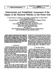
Figure 3-5. Localization process using Multilateration method of one RFID tag with three RFID Readers.

The theoretical solution of this method is explained in the next section in order to give a general idea of the Multilateration location approach. However, results are only valid in ideal conditions, and this particular solution is not able to solve some non ideal situations quite common in indoor environments. In Chapter 5, the posterior probability analysis is presented as one possible solution for solving the location of a RFID target tag in any situation by means of probabilistic approaches. 3.3.1 Theoretical analysis As it has been pointed out previously, when ideal conditions are supposed in the scenario, a simplification technique could be used in order to locate the RFID target tag. If all the distances are estimated with no errors, only one point of intersection will be found, and therefore, the location of the RFID target tag can be analytically calculated by applying basic trigonometric rules as it is explain below. With intention to simplify calculations, it will be assumed that the distance between each RFID Reader in the system and the RFID target tag is known. So, let us assume one scenario, where one RFID target node is located in (x,y) coordinates, and 3 RFID Readers, defined as ReaderA, ReaderB, ReaderC, are located in known coordinates. Note that, in this trigonometric approach, the definition of a coordinate system is completely needed to estimate properly the location of the RFID target tag. In order to simplify the system of equations, let us impose that ReaderA is located in the coordinate system origin, with coordinates (0,0), ReaderB is located in the horizontal axis with coordinates (xB,0) and the last, ReaderC is located in (xC,yC). Figure 3-6 shows graphically the RSS scenario considered.

15


y = f(x)


READERC (xC, yC)

DC

DA

DB

READERA (0,0) READERB (xB,0)

x

Figure 3-6. Definition of the system coordinates for Multilateration scenario.

If the distance between each RFID Reader and the RFID target tag is known, the location of the RFID target tag can be estimated by finding the intersection among 3 circles, centred in each RFID Reader with a radius equal to the distance estimated between the RFID Reader and the RFID target tag (Da, Db and Dc). Analytically, in a Cartesian coordinate system, a generic circumference of radius Di which is centred in the point (xi, yi) can be expressed as (3.1). (𝑥 − 𝑥𝑖 )2 + (𝑦 − 𝑦𝑖 2 ) = 𝐷𝑖 2

(3.1)

Figure 3-7 shows graphically the previous expression. TARGET (RFID TAG) (x,y)

y

Di READERi (xi, yi)

(y-yi)

yi (x-xi)

xi

x

Figure 3-7. Mathematical definition of a circle with radius equals to distance between RFID Reader and tag.

Therefore, applying the trigonometric expression for each circle and substituting the corresponding distances and locations for each one, the resulting expressions are (3.2), (3.3), and (3.4) respectively; 16


(𝑥 − 𝑥𝐴 )2 + (𝑦 − 𝑦𝐴 2 ) = (𝑥 2 + 𝑦 2 ) = 𝐷𝐴 2 𝑥 − 𝑥𝐵 2 + 𝑦 − 𝑦𝐵 2 = 𝑥 − 𝑥𝐵 (𝑥 − 𝑥𝐶 )2 + (𝑦 − 𝑦𝐶 2 ) = 𝐷𝐶 2

2

(3.2)

+ 𝑦 2 = 𝐷𝐵 2

(3.3) (3.4)

Then, if a system of three equations is considered, and taking into account that all the RFID Reader coordinates are known, it is possible to isolate both coordinates of the RFID target tag (x,y) as it is described below. First, if the square of D A and DB is subtracted, the obtained equation is (3.5); 𝐷𝐴 2 − 𝐷𝐵 2 = (𝑥 2 + 𝑦 2 ) − [ 𝑥 − 𝑥𝐵

2

+ 𝑦2] =

= (𝑥 2 + 𝑦 2 ) − [(𝑥 2 − 2x𝑥𝐵 + 𝑥𝐵 2 ) + 𝑦 2 = 2x𝑥𝐵 − 𝑥𝐵 2

(3.5)

Isolating the x coordinate is possible to obtain the expression (3.6);

2x𝑥𝐵 = 𝐷𝐵 2 − 𝐷𝐴 2 + 𝑥𝐵 2

→

x=

𝐷𝐵 2 − 𝐷𝐴 2 +𝑥 𝐵 2

(3.6)

2𝑥 𝐵

Once the x coordinate is isolated, the y coordinate can be calculated by applying the same method, but in this case, obtaining the difference of the distances squares between DA and DC and substituting x by its equality (3.7). 𝐷𝐴 2 − 𝐷𝐶 2 = (𝑥 2 + 𝑦 2 ) − [(𝑥 − 𝑥𝐶 )2 + (𝑦 − 𝑦𝐶 2 )] = (𝑥 2 + 𝑦 2 ) − [(𝑥 2 − 2x𝑥𝐶 + 𝑥𝐶 2 ) + (𝑦 2 − 2y𝑦𝐶 + 𝑦𝐶 2 )] = = 2x𝑥𝐶 − 𝑥𝐶 2 + 2y𝑦𝐶 − 𝑦𝐶 2

(3.7)

Isolating the second coordinate y is possible to deduce (3.8) and (3.9);

2y𝑦𝐶 = 𝐷𝐴 2 − 𝐷𝐶 2 − 2x𝑥𝐶 + 𝑥𝐶 2 + 𝑦𝐶 2 y=

𝐷𝐴 2 − 𝐷𝐶 2 − 2x𝑥 𝐶 + 𝑥 𝐶 2 + 𝑦 𝐶 2 2𝑦 𝐶

=

(3.8)

𝐷 2 − 𝐷 𝐴 2 +𝑥 𝐵 2 𝐷𝐴 2 − 𝐷𝐶 2 − 𝑥 𝐶 𝐵 + 𝑥𝐶+ 𝑦𝐶 2 𝑥𝐵

2𝑦 𝐶

(3.9)

So finally, it is possible to estimate the location of the RFID target tag as the equations (3.10) and (3.11). Figure 3-8 shows graphically the analytical results achieved in the previous analysis. 17


x= y=

𝐷𝐵 2 − 𝐷𝐴 2 +𝑥 𝐵 2

(3.10)

2𝑥 𝐵 𝐷𝐴 2 − 𝐷𝐶 2 − 𝑥 𝐶

𝐷 𝐵 2 − 𝐷 𝐴 2 +𝑥 𝐵 2 𝑥𝐵

+ 𝑥 𝐶 + 𝑦𝐶 2

(3.11)

2𝑦 𝐶

y = f(x)


READERC (xC, yC)

DC DB

DA

READERA (0,0) READERB (xB,0)

x

Figure 3-8. Analytical solution of the llocalization process using RSS Multilateration method.

The following sections will describe the performance of this location method in RFID systems and UWB communications. 3.3.2 RSS in RFID and UWB systems The RSS technique has been widely used in wireless location, and also in RFID systems due to its good features such as low complexity, and therefore, low cost of implementation (Homayoun Nikookar, 2008)(Zhou, Junyi, Shi, & Jing, July 2009). However, the localization accuracy suffers an important disadvantage when the system is deployed in a multipath scenario. Due to this effect, the received signal will have a high probability of degradation owing to multipath fading in each one of the RFID Readers, and therefore, the RSS parameter will be quite degraded declining the accuracy of the overall technique. In order to improve the accuracy of the location technique in RFID systems, a higher number of RFID Readers are used, and locations are combined constructively, reducing in this way the probability of error when locating the target node, and increasing the accuracy of the overall system. In this situation, the location technique is also known as Multilateration. The behaviour of the RSS location technique could be improved in indoor environments if it is combined with UWB technology. In fact, using UWB it is possible to avoid the multipath fading, or at least, reducing largely the probability of fading in multipath environments thanks to the high time resolution of the UWB signals (Homayoun Nikookar, 2008).

18


If the received signal is not affected by Multipath in the RFID Reader, the accuracy of the location technique increases considerably, and the correct selection of the channel model will be the main goal for achieving high accuracy in the RSS technique. 3.3.3 Conclusions To conclude, it is possible to see that the RSS technique is a good solution in RFID systems thanks to its low cost of implementation and low computational complexity. However, the behaviour of the RSS technique in indoor environment is directly affected by multipath fading when applied in RFID systems, and consequently, low accuracies are obtained by this location technique. If UWB is combined with RFID systems, multipath immunity could be achieved thanks to the high bandwidth resolution of the UWB, and therefore, the RSS technique becomes one solution for RFID indoor localization. Furthermore, if RSS is combined with other location method which accuracy improves using UBW signals, it is possible to improve the global accuracy of the system.

3.4 Triangulation with Angle of Arrival (AOA) Another classical technique for location in wireless environments is the Triangulation approach. It is also one of the most basic techniques to localize a RFID target tag, and it only requires two RFID Readers, or at least two RFID antennas connected to one RFID Reader, to localize the RFID target tag in 2-Dimensions. The triangulation technique is mainly based in estimating the Angle of Arrival (AOA) among the RFID target tag and the RFID Readers. It is only required to known the distance between two RFID Readers and both angles of incidence between each RFID Reader and the RFID target tag to estimate the RFID target tag location. Figure 3-9 depicts the principles of the Angle-of-Arrival technique graphically. Two RFID Readers are placed in known locations and the RFID target tag location is estimated by calculating the intersection of two lines coming from each RFID Reader to the RFID target tag. The theoretical analysis of the location is described in the following section. Note that, unlike in the RSS method, the distance between the RFID Readers and the RFID target tag is not estimated, and only the Angle of incidence must be detected to estimate the location.

19


TARGET (RFID TAG)

θα

θβ

READERA

READERB DAB

Figure 3-9. AOA technique based on the intersection of two lines drawing from each RFID Reader to the RFID tag.

3.4.1 Theoretical approach Analytically, the location in the triangulation technique consist of applying the principles of trigonometric rules, but again, the complexity of this technique rely directly on the Angle of Arrival estimation. As previously, it will be supposed that the AOA parameter is correctly estimated in order to describe the analytical solution of the location and in the next lines the estimation of the AOA issue will be discussed. As a general idea, the Triangulation technique location consists of finding the trigonometric intersection between two lines in a coordinate system. To do that, it is first necessary to remember the generic expression of one straight line (3.21);

𝑦 = 𝑀𝑥 + 𝑁

(3.21)

Where M is the slope of the straight line, and N is the offset of the straight line, which actually refers to the intersection between the straight line and the y axis of coordinates. On the other hand, at least one point and one of the two parameters previously described must be known to define correctly the straight line equation. Specifically, in the triangulation technique, two RFID Readers are located in two known points, and the AOA between each RFID Reader and the RFID target tag is also known, which in fact becomes the slope of each one of the two straight lines. In order to simplify the analysis, let suppose that the coordinates of the ReaderA are (0,0), and the coordinates of the ReaderB are (xb,0), and let define the distance between both of the RFID Readers as DAB, and therefore, the distance between both Readers can be also expressed as (3.22);

𝐷𝐴𝐵 = 𝑥𝑏

(3.22)

20


Figure 3-10 depicts graphically the scenario considered for the Triangulation technique; y = f(x)


f1(x)

θα READERA (0,0)

f2(x)

θβ READERB (xb,0)

x

Figure 3-10. Graphical representation of the analytical solution using the AOA technique.

Note that, both angles of arrival are defined as θα and θβ in each ReaderA and ReaderB respectively. Having these initial conditions, the RFID target tag location can be analytically estimated as follows. The first step consist in finding the equation of the straight lines f1(x) and f2(x). Knowing the slope and at least one point of the line, both expressions can be deduced as follows;

𝑓1 (𝑥) = 𝑀1 𝑥 + 𝑁1

(3.23)

Knowing the slope of the straight line 𝑀1 = tan 𝜃𝛼 , and at least one point of the equation line, ReaderA (0,0); it can be deduced that; 0 = tan 𝜃𝛼 ∗ 0 + N1 → 𝑁1 = 0

(3.24)

𝑓1 (𝑥) = tan 𝜃𝛼 ∗ x

(3.25)

On the other hand, the same steps are followed to achieve the second straight line equation, f2(x), as it is expressed in (3.26);

𝑓2 (𝑥) = 𝑀2 𝑥 + 𝑁2

(3.26)

Again, the slope of the straight line 𝑀1 = tan 𝜃𝛽 , and at least one point of the equation line, ReaderB (xb,0); it can be deduced then; 21


0 = tan 𝜃𝛽 ∗ xb + N2 → 𝑁2 = − tan 𝜃𝛽 ∗ xb

(3.27)

𝑓2 (𝑥) = tan 𝜃𝛽 ∗ x − tan 𝜃𝛽 ∗ xb

(3.28)

Once both of the expressions are deduced, the intersection between them can be estimated matching both f1(x) and f2(x) expressions in the coordinates (x,y) of the RFID target tag.

𝑓1 (𝑥) = 𝑀1 𝑥 + 𝑁1 = 𝑓2 (𝑥) = 𝑀2 𝑥 + 𝑁2

(3.29)

tan 𝜃𝛼 ∗ x = tan 𝜃𝛽 ∗ x − tan 𝜃𝛽 ∗ xb

(3.30)

And the results of the RFID target tag location are shown in the following equations;

𝑥= 𝑦=

− tan 𝜃 𝛽 ∗x B tan 𝜃𝛼 −tan 𝜃 𝛽 − tan 𝜃𝛼 ∗tan 𝜃 𝛽 ∗x b tan 𝜃𝛼 −tan 𝜃 𝛽

(3.31) (3.32)

Next section will discuss the advantages and disadvantages of this location method in RFID systems and UWB communications. 3.4.2 AOA in RFID and UWB systems As it has been demonstrated, the AOA technique is an interesting alternative in RFID location systems, mainly because of the low complexity computation that it requires as well as its simplicity for estimating the target location. Specifically, only two RFID readers are needed in order to achieve the RFID target tag position, and as it happens in RSS, it is better to count on high number of RFID Readers to reduce the undesirable interference in the received signal due to the multipath effect. Additionally, the systems based on AOA measurements do not require knowing the loss propagation model or synchronization. On the other hand, AOA has lower accuracy in such cases where the RFID target tag is far from the reader nodes. This happens because a small error in the angle estimation supposes a large error in the far-off intersection of two lines. Besides, the AOA technique requires antenna arrays to detect the Angle of Arrival which increases remarkably the price and the complexity of the hardware. Moreover, the long-life expectancy of the RFID systems declines when using these components (Bouet & Santos, 2008). Unlike other location techniques, applying UWB technology in AOA will not improve the behavior and the accuracy of the system. The reason is that using antenna arrays in 22


RFID Readers will increase the complexity of transceivers, and therefore, the cost of the global system. In addition, the large bandwidth of UWB signals causes a large number of paths which results extremely difficult to determine the correct Angel of Arrival (Gezici, et al., July 2005). 3.4.3 Conclusions Unfortunately, the simplicity of the trigonometric approach of the AOA technique not compensate the drawback of complex hardware and calibration of antennas dependency, concluding that, this technique is not suited for low cost and low complex location systems such as RFID with UWB location.

3.5 K Nearest Neighbours (KNN) The KNN technique is also a typical location technique in RFID systems and mainly consists of calculating the RFID target tag location based on the proximity principle (Zhou, Junyi, Shi, & Jing, July 2009). First, the RFID Reader interrogates the RFID target tag in order to acquire the RSS metric. Afterwards, the RFID Reader compares the RSS received from the RFID target tag with the RSS received from the K nearest RFID reference tags. Finally the RFID target tag location is estimated by means of RSS comparisons. Note that this RFID reference tags are not RFID Readers, and therefore they do not process information, and so that, they can only reply to an interrogation from the RFID Reader. It is notable to highlight that the location of the RFID reference tags is known and is strategically distributed in some specific scenario. In fact, in the KNN technique, the RFID reference tags are usually placed in the scenario following known and basic grid patterns, as it is shown in the Figure 3-11;

R1

R4

R2

R3

R5

R6 T

R7

R8

R9

RSS1 RSS2 RSS3 RSS4 RSS5 RSS6 RSS7 RSS8 RSS9 RSST

READER

Reference RFID TAGS Target RFID TAG

Figure 3-11. Graphical representation of the interrogation process of one RFID Reader in a scenario with multiple RFID reference tags and one RFID target tag.

23


Moreover, to achieve the location, an analysis of the scenario must be done previously, and several measurements must be stored in a data base before localizing the RFID target tag. Once the RFID reference tags are fixed, the RFID Reader interrogates periodically the RFID reference tags in order to acquire periodical RSS parameters from the scenario. When the RFID target tag comes into the controlled scenario, RFID Readers acquires a new sample of RSS coming from the RFID target tag. Then, the algorithm estimates the position of the target based on the comparison of the K weighted RSS measures of reference tags with the unknown tag RSS measure. The analytical process of location can be consulted in the following section for a detailed comprehension of the technique. 3.5.1 Theoretical approach Analytically, the proximity principle is applied through the periodical measurements of the RSS from RFID reference tags in the scenario as it is described below. Let suppose that there are 9 RFID reference tags placed in a square grid, and one RFID target tag comes into the scenario. Let also suppose that, there is only one RFID Reader, and it is placed out of the square grid (Figure 3-11). With intention to locate the RFID target tag, the RFID Reader must interrogate the 9 RFID reference tags and the RFID target tag, at least once, in order to achieve the overall RSS metrics from all RFID tags of the scenario. The analytical approach consist of determining the difference of the obtained RSS parameters by means of similar way as the Euclidean distance measures the difference in distance between two points. In fact, what this technique computes is the Euclidean distance of the Received Signal Strengths as it is expressed in the equation (3.33), instead of computing the difference between the distances of both points.

𝐸𝑢𝑟 =

𝑁 𝑛 =1

𝑆𝑆𝑛𝑟 − 𝑆𝑆𝑛𝑡 =

𝑁 𝑛 =1 (𝑆𝑆𝑛𝑟

− 𝑆𝑆𝑛𝑡 )2

(3.33)

Where n is the number of RFID readers in the system, SSnr is the Signal Strength of the r RFID reference tags received in the n RFID Reader with r={1,2,3...M}, and SSnt is the Signal Strength of the t RFID target tag received in the n RFID Reader. In current case, only one RFID Reader is considered, N=1, and therefore, the Euclidean expression becomes (3.34);

𝐸𝑡𝑟 = 𝑆𝑆𝑟 − 𝑆𝑆𝑡 = ∆𝑅𝑆𝑆𝑟𝑡

(3.34)

24


And r = {1,2,3....9} because only 9 RFID reference tags are considered in the particular scenario. Figure 3-12 shows graphically the concept of the Euclidean distance when it is applied with RSS measurements. K Nearest Neighbours = 4 R2

R1

R4

R3

R5

R6 ΔRSS6-T

ΔRSS5-T

RSS5 RSST

T

ΔRSS8-T

RSS6

RSS8

ΔRSS9-T

RSS9

R7

R8

READER

R9

Figure 3-12. Localization process considering four Nearest Neighbors using Euclidean distance information.

Note that, only the K nearest neighbours are considered in the previous estimations. K is a parameter which must be configured in the system initially and reflects the number of neighbours, or RFID reference tags that will be taken into account when computing the RSS differences. If K is equal to 1, the location of the RFID target tag is directly supposed to be the same as the RFID reference tag with the most similar RSS. Otherwise, with K higher than one, an average of the distances using the weight of the K RFID reference tags must be done. The weighting of the K nearest distances is basically the percentage of proximity of each one of the K nearest RFID reference tags with the RFID target tag. The weight of each RFID reference tag is estimated as it is expressed in (3.35);

1

𝑤𝑢𝑟 =

𝐸𝑢𝑟 2 𝑘 1 𝑟=1 𝐸 2 𝑢𝑟

(3.35)

Finally, the RFID target tag location can be estimated as the sum of the product between the RFID reference tag coordinates and the weights of each one of them;

𝑥, 𝑦 =

𝑘 𝑖=1 𝑤𝑖 (𝑥𝑖 , 𝑦𝑖 )

(3.36)

As an example, let imagine a situation where K=4, so four RFID reference tags are the neighbours of the RFID target tag (Figure 3-13). Let also suppose that, the Euclidean 25


distance of each one of them is the same, and therefore, the value of the weight of each RFID reference tag will be w1= w2= w3= w4=0,25 (25%). If the four RFID reference tags are situated in a coordinate system as it is shown in the Figure 3-13, the location of the RFID target tag could be estimated as it is expressed in the equation (3.37) and (3.38);

y

(0,1)R1

yT=?

R2 (1,1) T

(0,0) R4

R3 (1,0) xT=?

x

Figure 3-13. Simple example of KNN technique with four RFID Reference tags.

4

𝒙𝑻 =

𝑤𝑖 𝑥𝑖 = 𝑤1 𝑥1 + 𝑤2 𝑥2 + 𝑤3 𝑥3 + 𝑤4 𝑥4 𝑖=1

= 0,25 ∗ 0 + 0,25 ∗ 1 + 0,25 ∗ 1 + 0,25 ∗ 0 = 𝟎, 𝟓 (3.37) 4

𝒚𝑻 =

𝑤𝑖 𝑦𝑖 = 𝑤1 𝑦1 + 𝑤2 𝑦2 + 𝑤3 𝑦3 + 𝑤4 𝑦4 𝑖=1

= 0,25 ∗ 0 + 0,25 ∗ 1 + 0,25 ∗ 1 + 0,25 ∗ 0 = 𝟎, 𝟓 (3.38)

Once the location method is exposed, the advantages and disadvantages of implementing it in RFID systems and UWB communications will be discussed in the following sections. 3.5.2 KNN in RFID and UWB systems This location technique is a good candidate location method in RFID systems due to the fact that it requires a high number of reference points, and the low cost of the RFID reference tags makes viable to use it in RFID systems. In this technique, the distance between reference points determines the accuracy. Note that, one of the main feature of this method in RFID is the possibility of estimating the RFID target tag location without knowing the channel model of the environment. A kind of average with weightings is carried out in order to average the location of the RFID target tag, by means of the Euclidean distance between receiver RSS.

26


However, the quality of the received RSS will specify the accuracy of the system, and if the indoor channel depredates the transmitted signal, the probability of having high accuracies will decline considerably. Let us suppose a simple KNN scenario where only one RFID Reader is deployed, if this RFID Reader receives incorrectly the RSS from the RFID target tag due to the channel behaviour, then the RFID Reader will estimate the RFID target tag in a wrong position in the grid. In order to avoid this problem, it is advisable to deploy more than one RFID Reader to get diverse RSS measurements from RFID target tag. As happened in the previous location techniques, when applying UWB in RFID location for indoor environments, the signal could becomes immune to the multipath fading. That means the probably of one reader detect a target with a wrong RSS, and therefore, estimate it in an uncorrected range of K nearest neighbours is lower than in a system without UWB technology. 3.5.3 CONCLUSIONS The KNN method is a method which calculates the target’s location in one step without determining the distance, angle or time of the target from the readers and reference points. In addition, the method, which is implemented in RFID systems, could be improved if UWB technology is applied thanks to less sensitive to the fading and multipath effect.

3.6 Multilateration with Time Difference of Arrival (TDOA) There are other location techniques that rely on time based metrics in order to localize the target. Two of them are the Time of Arrival (TOA) technique and the Time Difference of Arrival (TDOA) technique. In the first one, the RFID Readers interrogate the RFID target tag. Afterwards, the time of arrival is computed in each of the RFID Readers, instead of computing other metrics such as the RSS or the AOA. As the propagation time is proportional to the distance, the intersections of three circles in a similar way to the RSS method can be used in order to localize the RFID target tag. However, this technique requires full synchronization of both transmitter and receiver, and as it is mentioned in (Homayoun Nikookar, 2008), 1 microsecond of inaccuracy could translate in an error of more than 300m when it is applied in UWB. So it is not viable to apply in RFID systems due to the fact that it is very complex to synchronize the RFID target tag with the RFID Readers. The other time base approach, the TDOA technique, is similar to the TOA because it also uses the time of arrival of the interrogation process. However, difference of arrival time between two different points is computed, and therefore, the system does not require to be synchronized completely. In fact, it only requires receiver synchronization, so that, in RFID systems it, is only necessary to synchronize the RFID Readers, but not the RFID target tag. The TDOA technique consists of estimating the position of the RFID target tag by means of the Time Difference metric. It requires, at least three RFID Readers, like the RSS technique, in order to achieve 2-Dimensions localization and it is banked on 27


calculating the hyperbolic intersection of at least two hyperbolas through Time Difference measurements. The process for determining the RFID target location is divided in two steps. First, each RFID Reader interrogates the RFID target reader in order to get the Time of Arrival metric. Then, each TOA metric is processed and converted into a Difference Time value. The analytical conversion results in one hyperbola by each pair of RFID Readers. By intersecting at least two hyperbolas is possible to estimate the target position. The next section describes in detail the analytical process of the TDOA Multilateration technique with three RFID Readers. 3.6.1 Theoretical Analysis Analytically, the Multilateration approach with TDOA metrics is more difficult to analyze than the previous three location techniques explained in the current chapter. The main reason is the non lineal behaviour of the general expression of the theoretical analysis, and therefore, the solution of the location requires more difficult approaches. Let deduce first, the general relation between the Difference time and the coordinates of the three RFID Readers. Let suppose that three RFID Readers are located in one coordinates system with coordinates (x1,y1), (x2,y2) and (x3,y3) and one RFID target tag comes into the coverage area of the RFID Readers. The interrogation of each RFID target tag will give one Time of Arrival measurement in each RFID Reader. Knowing that, the distance between two points is proportional to the Time of Arrival, the expression of the distance Ri from each RFID Reader to the RFID target tag, supposing i = {1,2,3} number of RFID Readers, is expressed as (47), being (x,y) the position of the RFID target tag.

𝑅𝑖 = 𝑐 · 𝑡𝑖 =

𝑥𝑖 − 𝑥

2

+ 𝑦𝑖 − 𝑦

2

=

𝑥𝑖 2 − 2𝑥𝑖 𝑥 + 𝑥 2 + 𝑦𝑖 2 − 2𝑦𝑖 𝑦 + 𝑦 2

(3.39)

Where ti is the Time of Arrival (TOA) between the RFID target tag and the RFID Reader, and c is the speed of light. Afterwards, the Time Difference of Arrival (TDOA) time can be expressed as (3.40);

𝑅𝑖,1 = 𝑐 · 𝜏𝑖,1 = 𝑅𝑖 − 𝑅1 =

𝑥𝑖 − 𝑥

2

+ 𝑦𝑖 − 𝑦

2

−

𝑥1 − 𝑥

2

+ 𝑦1 − 𝑦

2

(3.40)

Where Ri,1 is the distance between the RFID Readersi,1 , and τi,j is the Time Difference (TDOA) between both RFID Readers. Note that, R1 is considered the distance between the RFID target tag and the RFID Reader where the signal arrives first, and it will be suppose to be another unknown factor from now on. Finally, the analytical solution of the location is the intersection between at least two hyperbolas and different methods for achieving this solution can be found in the literature. Each one of them have different features in terms of accuracy, complexity or

28


equation derivation, and any one of them could be implemented depending on the requirements or the initial conditions of the system. As an example, some of them approach to linear system the hyperbola equations by the Taylor-series expansion method (FOY, MARCH 1976), and some others, such as the Fang’s method (MSSAN ELKAMCHOUCHI, 2005)(Stefanski, September, 2009), transform the non linear expressions in a linear system of equations before solving the system. The Fang’s method is quite suitable for low complex systems with three RFID Readers and the analytical derivations of this method are explained in the following section. 3.6.2 The Fang’s method as solution for location in TDOA The first step in the Fang’s method consist of transform in a linear behaviour the non linear expressions of the hyperbolas by means of some mathematical transformations before solving the location, as it is described below; Knowing that (3.40) is non linear, it is possible to change the order of the distances, and apply the square in both sides of the expressions, achieving (3.41) and (3.42);

(𝑅𝑖,1 + 𝑅1 )2 = 𝑅𝑖 2

(3.41)

𝑅𝑖,1 2 + 2𝑅𝑖,1 𝑅1 + 𝑅1 2 = 𝑅𝑖 2 (3.42)

Then, introducing equation (3.41) in (3.42), it is obtained (3.43);

𝑅𝑖,1 2 + 2𝑅𝑖,1 𝑅1 + 𝑅1 2 = 𝑥𝑖 2 − 2𝑥𝑖 𝑥 + 𝑥 2 + 𝑦𝑖 2 − 2𝑦𝑖 𝑦 + 𝑦 2 (3.34)

Finally, finding the difference between (3.34) and (3.39), applying i=1 in the second one, it is possible to obtain (3.44);

𝑅𝑖,𝑗 2 + 2𝑅𝑖,𝑗 𝑅𝑗 + 𝑅𝑗 2 = 𝑥𝑖 2 − 2𝑥𝑖 𝑥 + 𝑥 2 + 𝑦𝑖 2 − 2𝑦𝑖 𝑦 + 𝑦 2 𝑅1 2 = 𝑥1 2 − 2𝑥1 𝑥 + 𝑥 2 + 𝑦1 2 − 2𝑦1 𝑦 + 𝑦 2

(3.44)

Resulting in (3.45);

𝑅𝑖,1 2 + 2𝑅𝑖 ,1 𝑅1 = (𝑥𝑖 2 − 2𝑥𝑖 𝑥 + 𝑥 2 + 𝑦𝑖 2 − 2𝑦𝑖 𝑦 + 𝑦 2 ) − 𝑥1 2 − 2𝑥1 𝑥 + 𝑥 2 + 𝑦1 2 −

2𝑦1𝑦+ 𝑦2=(𝑥𝑖2−𝑥12)+(𝑦𝑖2−𝑦12)+2𝑥−𝑥𝑖+ 𝑥1+2𝑦 −𝑦𝑖+ 𝑦1)

(3.45) Knowing that (𝑥𝑖 −𝑥1 ) is equal to xi,1 and (𝑦𝑖 −𝑦1 ) is equal to yi,1 is possible to express the previous equation as (3.46); 29


𝑅𝑖,1 2 + 2𝑅𝑖,1 𝑅1 = 𝑥𝑖 2 + 𝑦𝑖 2 − 2𝑥𝑥𝑖,1 − 2𝑦𝑦𝑖,1 −𝑥1 2 −𝑦1 2

(3.47)

Let suppose now, that the previous RFID Readers1,2,3 are placed in the coordinates (0,0), (x2,0) and (x3,y3) respectively as it is shown in Figure 3-14. Due to the specific positions of the RFID Readers, the previous expressions can be simplified as it is shown in (3.48), (3.49) and (3.50);

𝑅1 = 𝑐𝑡1 =

2

𝑥1 − 𝑥

+ 𝑦1 − 𝑦

2

=

𝑥2 + 𝑦2

(3.48)

𝑥𝑖,1 = 𝑥𝑖 − 𝑥1 = 𝑥𝑖

(3.49)

𝑦𝑖,1 = 𝑦𝑖 − 𝑦1 = 𝑦𝑖

(3.50)

And therefore, reducing the (3.47) expression in the following one (3.51); 2𝑅𝑖,1 𝑅1 = 𝑥𝑖 2 + 𝑦𝑖 2 − 2𝑥𝑥𝑖 − 2𝑦𝑦𝑖 − 𝑅𝑖,1 2

(3.51)

y = f(x)


READER3 (x3, y3)

R3

R2,3 R1 R1,3

R2

READER1 (0,0) READER2 (x2,0)

R1,2

x

Figure 3-14. Graphical definition of the system coordinates and distances between RFID Readers and tag.

Finally, applying the expression in each of the RFID Readers, it is obtained (3.52) and (3.53);

2𝑅2,1 𝑅1 = 𝑥2 2 − 2𝑥𝑥2 − 𝑅2,1 2

→ 2𝑅1 =

2𝑅3,1 𝑅1 = 𝑥3 2 + 𝑦3 2 − 2𝑥𝑥3 − 2𝑦𝑦3 − 𝑅3,1 2

→

2𝑅1 =

𝑥 2 2 −2𝑥𝑥 2 −𝑅2,1 2 𝑅2,1 𝑥 3 2 +𝑦3 2 −2𝑥 𝑥 3 −2𝑦 𝑦3 −𝑅3,1 2 𝑅3,1

(3.52) (3.53)

30


Equating the previous both equations in (3.54), it is possible to obtain an expression such as (3.55);

𝑥 2 2 −2𝑥𝑥 2,1 −𝑅2,1 2 𝑅2,1

=

𝑥 3 2 +𝑦3 2 −2𝑥𝑥 3 −2𝑦𝑦3 −𝑅3,1 2 𝑅3,1

𝑦 = 𝑔𝑥 + 𝑕

(3.54)

(3.55)

Where g and h are respectively (3.56) and (3.57);

𝑔= 𝑕=

𝑅31

𝑥2 𝑅 21

− 𝑥3

𝑦3

−

𝑥3

(3.56)

𝑦3

2 −𝑅 𝑅 𝑥 32 + 𝑦32 −𝑅31 31 21 1+

𝑥2 2 𝑅 21

2𝑦3

(3.57)

Then, knowing that (3.58);

2𝑅2,1 𝑅1 = 𝑥2 2 − 2𝑥𝑥2 − 𝑅2,1 2 𝑅1 =

𝑥2 + 𝑦2

(3.58)

It can be substituted y by the previous expression, in order to obtain (3.59) and (3.60);

2𝑅2,1 𝑥 2 + 𝑦 2 = 𝑥2 2 − 2𝑥𝑥2 − 𝑅2,1 2 𝑦 = 𝑔𝑥 + 𝑕

(3.59)

2𝑅2,1 𝑥 2 + (𝑔𝑥 + 𝑕)2 = 𝑥2 2 − 2𝑥𝑥2 − 𝑅2,1 2

(3.60)

If afterwards, the square is applied in both sides of the equation, and the expression is divided by (2𝑅2,1 )2 quadratic expression such as (3.61) can be found; 𝑑𝑥 2 + 𝑒𝑥 + 𝑓 = 0

(3.62)

Where d,e and f are respectively (3.64), (3.65) and (3.66);

31


𝑑 = 1 + 𝑔2 −

𝑥2

𝑥2

𝑒 = 2𝑔𝑕 + 𝑥2 𝑓 = 𝑕2 −

(3.64)

𝑅21

𝑅21

2

−1

2 𝑥2 2 −1 𝑅 21

4

(3.65)

(3.66)

Finally, by applying the solution of a quadratic equation, and taking into account only the positive term of the solution, the x coordinate can be deduced as (3.67);

𝑥=

−𝑒+ 𝑒 2 −4𝑑𝑓 2𝑑

(3.67)

The second location coordinate y can be deduced if the x coordinate expression is applied in the expression (3.67). 3.6.3 TDOA in RFID and UWB systems The TDOA metric in RFID systems has not been widely implemented as other metrics such as RSS, due to the difficulties of detecting the Time of Arrival. Note that the RFID Readers must be well synchronized in time, and then, the moment of arrival of the system must be precisely detected in order to avoid estimation errors. Multipath may introduce time measurement errors when not Light-of-sight (LOS) is present in the system, causing estimation errors in the location. However, if UWB is applied in RFID systems with these techniques, high accuracy results may be achieved. In UWB systems, TDOA is a good location technique due to the fact that, TDOA is based on time approaches, and the time resolution of UWB is higher than the other radiofrequencies used in RFID systems (UHF, HF and LF) due to the ultra wideband range of operation. Moreover, one of the strengths of UWB is its low sensitive to multipath problems and therefore, estimation errors in indoor environments using RFID systems with UWB can be avoided, improving the accuracy of the overall system. 3.6.4 Conclusions So in this section, the TDOA time based approach has become the best option of time based approaches when UWB in RFID systems are used. High accuracy and relatively low computational complexity could be achieved depending on the scenario (three RFID Readers) if the Fang’s method is applied for determining the location of the target. Despite TDOA Multilateration metric could report really good results in location systems when using with UWB technology, it is possible to improve its performance by combining it with the previous Multilateration RSS location method, obtaining the RSS/TDOA hybrid location scheme. 32


3.7 Conclusions In the present chapter, some classical location methods used in wireless communications have been mathematically analyzed in ideal conditions. However, adverse effects are present in real environments. Unfortunately, when non-ideal conditions affect the received metric, wrong measures are obtained, and consequently, simple trigonometric formulas are not possible to be used in real location methods. As a result, it is completely necessary to understand which effects are present in indoor channels with the intention to find later location methods which make RFID target tag position possible. Thus, the following chapter is devoted to describe the mathematical models which can determine the behaviour of an indoor radio-propagation channel.

33


34

4 INDOOR RADIO-PROPAGATION CHANNEL MODELS

4 INDOOR RADIO-PROPAGATION CHANNEL MODELS Wireless communications usually suffer non ideal behaviours when transmitted through the communication channel, and its transmission from the emitter to the receiver will directly depend on propagation channel conditions. Several channel model approaches have been proposed in the literature depending on the channel conditions. The first and classical approach to estimate the behaviour of the wireless channel over a radio signal consist of considering an ideal scenario were only free space losses and white Gaussian noise affects directly the transmitted signal. When this ideal situation is considered, the received power is attenuated by the square of the distance following the free space losses factor and therefore the received signal can be easily estimated theoretically. However, when considering real systems, where the environment conditions are not ideal, not only the propagation losses in free space must be considered, but also other non ideal behaviour of the signal have to be taken into account owing to get accurate results. A specifically in indoor environment, multipath is the most important phenomenon to be contemplated in indoor channels and its behaviour is unpredictable. Thus, in order to recover the original emitted signal it is necessary to use statistics and probabilistic channel models that estimate mathematically the channel behaviour. For this reason, the aim of the following sections is to demonstrate that indoor channels, especially those suffering large number of multipath, can be approached as Rician or Rayleigh channel models, explaining first multipath effect in fading channels, and after, Rician and Rayleigh probability distributions.

4.1 Fading in wireless channels Due to the non ideal behaviour of the wireless channels, the reached signal in the receiver is not exactly the same as the transmitted one. There are several physical reasons explaining that fact such as diffractions, reflections and refraction caused all of them by obstacles, walls and buildings. The combination of these physical effects will directly affect the received signal. Analytically, the unpredicted behaviour of the received signal in any wireless channel can be estimated taking into account three different phenomena which are known as propagation losses, slow fading and fast fading. However, before entering in detail in each one of them, it is important to remember some wireless electromagnetic concepts. The electromagnetic radiation is the phenomenon of propagating electromagnetic waves in a vacuum or in matter.

35


The electromagnetic wave is composed by two components, the electric field E and the magnetic field H. These fields oscillate in phase perpendicular to each other and both propagate perpendicular to the direction of energy propagation. Specifically in telecommunications, waves are used to transport information within different parameters such as amplitude, phase and frequency. Therefore, any change of any one of these three information parameters may result in losses of information, or degradation of the communication, and for this reason, channel models are needed in order to avoid unknown behaviours of the transmissions. The first no ideal phenomenon are the propagation losses. Considering a classical and ideal approach in wireless system, the attenuation of the communication is modelled as free space losses where the power of the received signal decreases proportional to the square of the distance. However, another physical phenomenon will also affect the signal in real environments known as fading. As it has been described before, fading refers to random deviations of the transmitted signal when travelling through a channel. However, these deviations could be originated by two kinds of fading, known as slow and fast fading. The slow fading, or shadowing, is mainly caused by the presence of obstacles in the environment, decreasing the ideal expected attenuation of the Line-of-sight (LOS) component (free space losses). In fact, it refers to slow deviations of the transmitted signal in time, or space, and it usually follows a log-normal distribution or a normal distribution, depending on if the power is expressed in lineal (mW or W) or in logarithmic (dBm or dBW) unities respectively. Normal distribution, also known as Gaussian distribution, is expressed as (4.1) and can be graphically depicted as in Figure 4-1 (Homayoun Nikookar, 2008).

𝑓 𝑟 =𝜎

1 2𝜋

𝑒

−

𝑥−𝜇 2 2𝜎 2

𝑟≥0

(4.1)

where μ is the average expected power resulting from Friis formula (in dBm or dBW) in free space propagation model, and the variance σ2 depends on the probability that electromagnetic waves suffers more or less attenuation due to obstacles during the propagation.

Figure 4-1. Example of a Normal probability function with generic mean and deviation.

36


In the other hand, fast fading, or multipath fading, creates continuous changes in the behaviour of the received signal as a consequence of fast time variations due to reflections, refractions and diffractions of the environment. Figure 4-2 shows graphically the effects of the channel when propagation losses and fading affects the transmitted signal in a generic communications channel.

Figure 4-2. Graphical explanation of the propagation losses behavior in fading channels.

As a conclusion, in indoor environments the received signal will be the sum of different paths attenuated and delayed in time, despite the origin is the shadowing, reflexions, refractions and diffractions. Finally, the receiver must deal with combination of independent paths which can be theoretically expressed as multipath. Therefore, it becomes absolutely necessary to know details of this effect and use the proper time-variant multipath channel models for dealing with multipath fading. The next section describes a theoretical analysis of the effects of multipath over a wireless transmitted signal.

4.2 Multipath effect analysis With the purpose of clarifying the effect of the multipath fading in indoor environments, it will be analytically studied the concept using electromagnetic theory, knowing that the multipath is caused by the combination of multiple paths, or the sum of multiple electromagnetic waves, getting to the receiver. Consider an electromagnetic signal expressed as (4.2);

𝑠 𝑡 = 𝑅𝑒 𝑏(𝑡)𝑒 𝑗 2𝜋 𝑓0 𝑡

(4.2)

Where s(t) is the signal to be transmit to the medium, f0 is the carrier frequency and b(t) is the band-base signal. If the signal (4.2) is scattered through a medium with multiple propagation paths, the receiver will reach the next band-pass signal (4.3), where θn(t) is the instant phase, τn is the delay and αn is the attenuation of the nth path:

37


𝑟 𝑡 = 𝑅𝑒

𝑛

𝛼𝑛 (𝑡)𝑏 𝑡 − 𝜏𝑛 (𝑡)𝑒 −𝑗 𝜃𝑛 (𝑡) 𝑒 𝑗2𝜋 𝑓0 𝑡 𝜃𝑛 𝑡 = 2𝜋𝑓0 𝜏𝑛 (𝑡)

(4.3)

Focusing on the term θn(t), if τn = 1/fc, the resulting phase of the component nth will be multiple of 2π, on the contrary, the phase will be reached between [0,2π). Finally, with the intention of characterizing the channel, if the expression (4.3) is carry to base-band (4.4), and therefore, the b(t) signal is replaced by delta function, the result is the time-variant impulse response of the channel (4.5). Note that the channel behaviour is constantly changing, a then it is not possible to model it as a fixed impulse response.

𝑟 𝑡 = 𝑅𝑒 𝑕 𝜏; 𝑡 =

𝑛 𝑛

𝛼𝑛 (𝑡)𝑒 −𝑗 𝜃𝑛 (𝑡) 𝑏 𝑡 − 𝜏𝑛 (𝑡)

𝛼𝑛 (𝑡)𝑒 −𝑗 𝜃𝑛 (𝑡) 𝛿 𝜏 − 𝜏𝑛 (𝑡)

(4.4) (4.5)

Hence, the received signal will be the sum of all the components, delayed in time, from diverse paths with different amplitude and phase. Therefore in multipath channels, for instance in indoor environments, the expected signal is a train of copies from the original signal. Figure 4-3 depicts an example of received signal if it is transmitted a pulse. Rx

Tx

Multipath channel

t0+τ1

t0+τ2

Figure 4-3. Example of time-spreading of one generic RF pulse in multipath environments.

Then, if it is assumed that there are a large number of paths n, or electromagnetic waves, travelling in the channel, and they are random and independent, the Central Limit Theorem (CLT) can be applied. The CLT theorem defines that the distribution of a large number of independent random variables with finite mean and variance, the model can be approximated as a normal (Gaussian) distribution. Thus, the time-variant impulse response of the channel can be expressed as a complex number (4.6), where x(t) and jy(t) are orthogonal independent random variables with the same mean and variance, or what is equivalent, they are circularly symmetric complex Gaussian random variables (David Tse, Feb. 2009).

𝑕 𝑡 = 𝑥 𝑡 + 𝑗𝑦 𝑡

(4.6)

38


Therefore, applying the CLT theorem to the previous received signal affected by multipath fading (4.3), the resulting expression is shown in (4.7) and Figure 4-4 depicts the received signal.

𝑟 𝑡 = 𝑅𝑒 (𝑥 𝑡 + 𝑗𝑦 𝑡 )𝑒 𝑗2𝜋 𝑓0 𝑡 = 𝑧 𝑡 cos⁡ (𝑤0 𝑡 + 𝜙 𝑡 ) 𝑧 𝑡 =

𝑥(𝑡)2 + 𝑦(𝑡)2

𝑦(𝑡)

𝜙 𝑡 = tan−1 𝑥(𝑡)

(4.7) (4.8)

jy(t)

z(t) ϕ(t) x(t)

Figure 4-4. Graphical representation of the components of a received signal when large number of paths is supposed.

Where r(t) is the new expression for received signal if the CLT is applied, and z(t) is the envelop of the received signal, and ϕ(t) is the resulting phase. As a result, the multipath channel satisfies the Rayleigh distribution definition as it will be described in the following section.

4.3 Rayleigh and Rician Models As it is known, Rayleigh distribution is applied, in probabilistic and statistic theory, when the components of a bi-dimensional vector are uncorrelated and normally distributed with equal variance and mean. Moreover, if no one of the multiple paths getting to the receiver is dominating over the others, then the Rayleigh approach can be applied for modelling the transmission channel. Knowing that, the received signal in indoor environments, with multipath propagation, is a complex vector with circularly symmetric complex Gaussian random components, is possible to express the probability density function (PDF) as a Rayleigh probability density function, see Figure 4-5 function a) Rayleigh PDF. Expression (4.9) is the generic formula of Rayleigh PDF, where z is the random variable which represents, in this case, the expected envelope of signal; and σ2 is the average power of the signal.

39


𝑧

𝑓𝑟 𝑧, 𝜎 =

𝜎2

2 −𝑧

2𝜎 2

𝑒

𝑧≥0

(4.9)

Otherwise, if one of the multiple paths that reach the receiver is dominant over the others, for instance a Line-of-Sight component, then the Rician model must be applied. Generally, this LOS component is the sum in phase between LOS and ground reflected components. Now, the received signal will be the sum of the multipath components plus an extra electromagnetic wave in LOS equal to 𝑏(𝑡)𝑒 𝑗 𝜃0 𝑡 , giving as a result, the expression (4.10), where α is the free space attenuation and the phase of LOS component θ0 is uniformly distributed between [0,2π).

𝑟 𝑡 = 𝑅𝑒 𝛼𝑏(𝑡)𝑒 𝑗 𝜃0

𝑡

+

𝑛

𝛼𝑛 𝑡 𝑏 𝑡 − 𝜏𝑛 𝑡 𝑒 −𝑗 𝜃𝑛 (4.10)

𝑡

𝑒 𝑗2𝜋 𝑓0 𝑡

𝜃0 𝑡 = 2𝜋𝑓0 (𝑡)

As discussed in Rayleigh model, the multipath components are modelled as independent Gaussian random variables x(t) and jy(t) (4.7), but in Rician case the strong component of LOS adds a permanent amplitude in the real part (4.11).

𝑟 𝑡 = 𝑅𝑒 (𝛼𝑏 𝑡 𝑒 𝑗 𝜃0

𝑡

+ 𝑥 𝑡 + 𝑗𝑦 𝑡 )𝑒 𝑗2𝜋𝑓0 𝑡 (4.11)

Finally, the Rician probability density function (4.12) (Proakis, 2000) is a particular case of the Rayleigh pdf (4.9) and depends on the zero-order Bessel function (4.13).

𝑧

𝑓𝑟 𝑟 = 𝜎 2 𝑒 𝑘𝑧

1

𝐼0 (𝜎 2 ) = 2𝜋

−(𝑧 2 −𝑘 2) 2𝜎 2

𝜋 −𝜋

𝑘𝑧

𝑒𝜎2

𝐼0

cos 𝜙

𝑘𝑧

𝑧≥0

𝜎2

𝑑𝜙

(4.12) (4.13)

Where now, 𝜎 2 is the average power of the multipath received power (4.14), taking into consideration the expected average power of the signal, and the received power from the LOS wave. Note that in this channel model, a K parameter, known as the Rician factor, is included. It represents the strength of the dominant component compared to the multipath components, and it can be expressed as follows (4.15).

𝜎 2 = 𝑃𝑚 −

𝐴2 2

(4.14)

40

4 INDOOR RADIO-PROPAGATION CHANNEL MODELS 𝐴2

𝐾 = 2𝜎 2

(4.15)

It is important to note that, if K equals to 0, then the Rician model becomes a Rayleigh model, as it can be deduced from the previous Rician distribution equation (4.12) when K=0. In the same sense, if K tends to infinite, then the probability distribution becomes a Gaussian distribution, as it depicts Figure 4-5, where (a) is Rayleigh distribution, (b) is Rician distribution and (c) is Gaussian or log-normal distribution;

Figure 4-5. Distribution models in fading channels. (a) Rayleigh, (b) Rician, (c) Gaussian

4.4 Conclusions Concluding the indoor wireless channel, multipath fading is the most important effect to be considered since it causes extra attenuation and energy-spreading of the transmitted signal. Consequently, RFID location methods, which are based on Received Strength Signal (RSS) parameter, are not completely suited in these environments because of extra attenuations provide extra errors in the localization process. Apart from that, the time-spreading effect, originated by multipath, results difficult to evaluate the target’s location in RFID methods based on time approaches. Regarding the two channel models studied, it can be considered that the most appropriate channel model when using RFID systems in indoor environments with large density of antennas is the Rician model. On the contrary, if low density of antennas is deployed in the scenario, it is better to use the Rayleigh model due to the low probability to obtain a LOS component. Finally, RFID systems use Rayleigh methods instead of Rician models because, in analytical point of view, it is much easy to implement the Rayleigh functions than Rician ones.

41


42

5 MODIFIED LOCATION METHODS CONSIDERING CHANNEL MODEL INFORMATION

5 MODIFIED LOCATION METHODS CONSIDERING CHANNEL MODEL INFORMATION It is well known that wireless communications, especially in indoor environments, are hardly affected by interferences that could degrade seriously the transmitted signal, and consequently, decline the accuracy of an RFID location method. As it has been described in the previous chapter, an indoor channel affected by multipath can create multiple replicas of the initial transmitted signal, and therefore, the received metric in one specific RFID Reader would have a certain probability of being wrong, or simply, suffering a deviation of the theoretical received value. For that reason, simply geometrical location techniques described in Chapter 3 are not completely right when the received metrics are affected by multipath, and therefore, it is necessary to include statistical information about the channel behaviour inside the location technique. In this chapter, two location methods are extended with the proper probabilistic channel information in order to enable their proper operation in real multipath fading channels. The structure of the chapter has been divided in two blocks corresponding to the analytical study of each modified location method independently.

5.1

Extended RSS location method for Multipath channels

As it has been described, the goal of the project consists of combining one location method suited for RFID systems with another one suited for UWB positioning. As it has been studied, different location techniques are currently used in RFID systems, but the RSS one has been widely implemented thanks to its low cost and computational complexity. Moreover, it has the capability of improving the location accuracy when it is combined with another method, and consequently, it has been the selected location method suited for RFID systems. 5.1.1 Theoretical Study With the purpose of solving all the possible locations in indoor environments in a specific scenario, the RSS location method has been modified with the proper channel model based on the maximum a posteriori probability criterion as well as on the Bayesian rules. The maximum a posteriori probability is a probabilistic result of an uncertain situation, or a random event, taking into account an initial condition. It is based on the Bayes theorem which is expressed as (5.1):

43


𝑃 𝐴𝐵 =

𝑃 𝐵 𝐴 𝑃(𝐴)

(5.1)

𝑃(𝐵)

Where 𝑃 𝐴 𝐵 ) is the probability of obtaining A when B is given or fixed, and depends on the probability of getting B when A is given ( 𝑃 𝐵 𝐴 , which is known as the likelihood, the probability of A (P(A)), which is the a prior probability, and finally, the probability of obtaining B (P(B)), or data (5.2).

𝑃𝑜𝑠𝑒𝑟𝑡𝑖𝑜𝑟 𝑝𝑟𝑜𝑏𝑎𝑏𝑖𝑙𝑖𝑡𝑦 =

𝐿𝑖𝑘𝑒𝑙𝑖 𝑕𝑜𝑜𝑑 ∗𝑝𝑟𝑖𝑜𝑟 𝑝𝑟𝑜𝑏𝑎𝑏𝑖𝑙𝑖𝑡𝑦

(5.2)

𝑑𝑎𝑡𝑎

In the present project, this theorem is used to determine the most probable location of the RFID Target tag. Let us suppose first one scenario where only one RFID Reader and the RFID target tag are present. It is possible to define the probability of the RFID target tag of being located at a distance di when the interrogation of the RFID Reader i results in a received RSSi, as (5.5);

𝑃 𝑑 𝑅𝑆𝑆𝑖 =

𝑃 𝑅𝑆𝑆 𝑖 𝑑 ∗𝑃(𝑑 ) 𝑃(𝑅𝑆𝑆 𝑖 )

(5.5)

Where 𝑃(𝑑) is the prior distribution defined as the probability of the RFID target tag as being in at the distance d, and the data probability 𝑃(𝑅𝑆𝑆𝑖 ) is defined as the probability of receiving the RSSi value in the RFID Reader over all the possible distances of the RFID target tag. Assuming that 𝑃(𝑑) is uniformly distributed because of the probability of being in some location is equal for all locations, it can be assumed that 𝑃 𝑑 is a constant value for any possible distance. Moreover, 𝑃(𝑅𝑆𝑆𝑖 ) is the expected value of the RSSi for all posible distances as it is theoretically expressed in (5.6). Thus, the probability of receiving any 𝑅𝑆𝑆𝑖 value will be the same in all the possible locations and consequently 𝑃(𝑅𝑆𝑆𝑖 ) can be also expressed as a constant value.

𝑃 𝑅𝑆𝑆𝑖 =

∞ −∞

𝑃 𝑅𝑆𝑆𝑖 𝑑 · 𝑃 𝑑 𝑑𝑑

(5.6)

Then, the initial exression (5.7) can be simplified as (16) taking into account that the product of two constants gives a new constant value;

𝑃 𝑑 𝑅𝑆𝑆𝑖 = 𝐶𝑖 · 𝑃 𝑅𝑆𝑆𝑖 𝑑

(5.7) 44


Where Ci is a constant value and it is formed by the fraction between 𝑃 𝑑 and 𝑃(𝑅𝑆𝑆𝑖 ), and 𝑃 𝑅𝑆𝑆𝑖 𝑑 is the probability density function (pdf) of the Received Signal Strenght (RSSi) at a particular distance. The expression of the pdf of the RSS metric at a given location relies on the channel model and can be easily determine if the channel distribution is known. Let us consider that the indoor channel can be modeled as a Rayleigh distribution channel, noting that the same process is valid for the Rician Distribution. Then, it is possible to express the previous expression (5.7) as (5.8); 𝑅𝑆𝑆 𝑖 2 −

𝑃 𝑑 𝑅𝑆𝑆𝑖 = 𝐶𝑖 · 𝑓𝑅𝑆𝑆 𝑅𝑆𝑆𝑖 , 𝜎 = 𝐶𝑖 ·

𝑅𝑆𝑆 𝑖 𝜎2

2𝜎 2

𝑒

𝑅𝑆𝑆 ≥ 0

(5.8)

where σ2 is the averaged received power and depends on the distance d to the RFID reader, it is expressed in (5.9);

𝜎 2 = 𝑃𝑡 − 10 ∗ 𝑛 ∗ log(2𝑑)

(5.9)

Where Pt is the transmitted power of one RFID Reader, n is the path loss factor of the channel and the distance is multiplied by two due to the fact that the RFID target tag is passive and therefore the transmited RFID signal from one reader must travel twice the distance. On the contray, if the tag is active the distance will be only considered once. Analytically, the result of the pdf of the RFID target tag being located at a distance given RSSi, can be expressed as (5.10) and graphically represented as Figure 5-1.

𝑅𝑆𝑆 𝑖 2 −

𝑃 𝑑 𝑅𝑆𝑆𝑖 = 𝐶𝑖 ·

𝑅𝑆𝑆 𝑖 [𝑃𝑡 −10𝑛 log (2𝑑 )]2

2[𝑃𝑡 −10𝑛 log (2𝑑 )]2

𝑒

(5.10)

y  P d RSSi


READERA (0,0)

d

Figure 5-1. Probability density function of the distance given one RSS metric in one Reader when considering Rayleigh channel.

45


Applying the basics of trigonometric, the distance between two points can be calculated from the coordinates between both points as it was described in the previous section. Then, (5.10) can be expressed in terms of (x,y) coordinates as in (5.11);

𝑅𝑆𝑆 𝑖 2 −

𝑃 (𝑥, 𝑦) 𝑅𝑆𝑆𝑖 = 𝐶𝑖 ·

𝑅𝑆𝑆 𝑖

2[𝑃𝑡 −10𝑛 log (2 ∆𝑥 2 +∆𝑦 2 )]2

𝑒 2

(5.11)

[𝑃𝑡 −10𝑛 log (2 ∆𝑥 2 +∆𝑦 2 )]

Where ∆𝑥 and ∆𝑦 are the distances between the RFID Reader and the RFID target tag in a Cartesian coordinates system, and can be represented in 3-Dimension as it is shown in Figure 5-2; ReaderA (0,0)

y=f(x,y,σ)


y

x

Figure 5-2. . Probability density function of the coordinates given one RSS considering Rayleigh channel.

As the location of the RFID target tag must be done with at least three RFID Readers, three PDF similar to the previous expression (5.11) will be deduced for each RFID Reader. Therefore, the PDF of the RFID target tag being located at a distance will be given by a vector of RSSi,as it is shown below (5.12);

𝑃 𝑑 𝑅𝑆𝑆 =

𝑃 𝑅𝑆𝑆 𝑑 ∗𝑃(𝑑 ) 𝑃(𝑅𝑆𝑆 )

(5.12)

Where 𝑅𝑆𝑆 = 𝑅𝑆𝑆1 𝑅𝑆𝑆2 𝑅𝑆𝑆3 is the vector of RSS measurements reported by the three RFID Readers. Simplifying as in (5.7), (5.12) results in (5.13);

𝑃 𝑑 𝑅𝑆𝑆 = 𝐾 · 𝑃 𝑅𝑆𝑆 𝑑

(5.13)

Where K is the product of constants C1, C2 and C3 from each RFID Reader. Knowing that the RSSi of each RFID Reader are independent variables, expression (5.13) can be simplified in (5.14);

46


𝑃 𝑑 𝑅𝑆𝑆 = 𝐾 ·

3 𝑖=1 𝑃

𝑅𝑆𝑆𝑖 𝑑

(5.14)

Finally, the location of the RFID target tag can be found in the coordinates (x,y) which maximizes the previous function (5.14), as it is expressed in (5.15). Note that the distance depends on coordinates (x,y);

𝑚𝑎𝑥𝑃 𝑥, 𝑦 𝑅𝑆𝑆 = 𝑚𝑎𝑥 𝑘 · 𝑃 𝑅𝑆𝑆 𝑥, 𝑦

= 𝑚𝑎𝑥 𝑘 · (5.15)

𝑁 𝑖=1 𝑃

𝑅𝑆𝑆𝑖 𝑥, 𝑦

There are different methods to find analytically the coordinates of the RFID target tag location from (5.15). In (Yamamoto, Matsutani, Matsuki, Oono, & Ohtsuka, 2001) an algorithm, based on probability density function, is proposed to find the coordinates of the RFID target tag by solving the expression (5.15) deriving the Mean Square Error (MSE) function (5.16), where 𝜀 is the MSE function (5.17).

𝜕𝜀 𝜕𝑥

𝜕𝜀

= 0;

𝜕𝑦

= 0;

(5.16)

𝜀 = 𝐸 (𝑥 − 𝑥 )2 + (𝑦 − 𝑦)2 = 𝐸 𝑥 2 − 2𝑥 𝐸 𝑥 + 𝑥 2 + 𝐸 𝑦 2 − 2𝑦𝐸 𝑦 + 𝑦 2 (5.17)

The results of equating the partial derivations of the MSE to zero results in the estimated solution of the RFID target tag (5.18) and (5.19).

𝑋=𝑥=𝐸 𝑥 =

∞ 𝑥𝑃 −∞

𝑌=𝑦=𝐸 𝑦 =

∞ −∞

𝑥 𝑟 𝑑𝑥 =

𝑦 𝑃 𝑦 𝑟 𝑑𝑥 =

∞ 𝑥 −∞ ∞ −∞

∞ −∞

𝑦

𝑃 𝑥, 𝑦 𝑅𝑆𝑆 𝑑𝑦 𝑑𝑥

∞ −∞

𝑃 𝑥, 𝑦 𝑅𝑆𝑆 𝑑𝑥 𝑑𝑦

(5.18) (5.19)

Where X and Y are the RFID target tag estimated coordinates and 𝑅𝑆𝑆 is the vector of the received RSSi signals from the three RFID Readers. Note that in (5.18) and (5.19), x and y refers to the integrating variables, while in (5.17) refer to the true value of the RFID target tag. Another possibility consist directly of deriving partially (5.15) for x and y equating then to zero (5.20). The isolation of both coordinates x and y will solve the system of equations, and therefore the RFID target tag localization.

0=

𝑑 𝑘∗𝑃 𝑅𝑆𝑆 𝑑 𝑑𝑥

;

0=

𝑑 𝑘∗𝑃 𝑅𝑆𝑆 𝑑 𝑑𝑦

(5.20)

47


However, deriving expression (5.20) and finding both x and y coordinates is not trivial because it includes the product of three PDF, each one of them with two variables (x,y). To conclude, it can be deduced that the modified location method includes all possible all possible effects of multipath fading channels and the solution of the estimated location can be found analytically in any situation. As an example, let consider two common situations where the RSS trigonometric technique is not able to estimate the position of the RFID target tag. 1) Three circles intersecting in more than one point Figure 5-3 2) Any circle intersects with the other ones Figure 5-4

y = f(x)


READERC

READERA READERB

x

Figure 5-3. One example of RSS location technique when more than one intersection occurs between three circles. y = f(x)

READERC TARGET (RFID TAG) (x,y)

READERA READERB

x

Figure 5-4. . One example of RSS location technique when non intersection occurs between three circles.

The reason is that the trigonometric technique is not able to find one solution in these situations. For that reason, the modified RSS location method has been proposed. The resulting PDFs of the previous examples with the modified RSS location method are depicted in Figure 5-5.

48


Figure 5-5. Graphical representation of the three PDF from each RFID Reader in the modified RSS location method; Left picture is first example and Right picture is the second one.

Now, the the previous circles become probabilistic functions depending on the location of the RFID target tag, and the solution of the location is not the intersection of them, but the product of PDFs. The resulting PDF is shown in Figure 5-7 for the previous examples;

Figure 5-6. Graphical representation of the resulting PDF product; Left picture is the first example and Right picture is the second one.

Therefore, the estimated location belongs to the maximum probable location inside the resulting PDF. 5.1.2 Theoretical evidences of the location error source The modified RSS location method relies on the principles of the PDF algorithm from (Yamamoto, Matsutani, Matsuki, Oono, & Ohtsuka, 2001). This algorithm consists of estimating the target’s position by means of calculating the PDF in each Reader of the target’s location. Applying the proper channel distribution, and the maximum posteriori probability approach it has been demonstrated that the both (x,y) coordinates of the target can be estimated from the expected value in x and y of the product of all the PDF in each Reader, as it is shown in (5.21) and (5.22).

𝑋=𝐸 𝑥 =

∞ −∞

𝑥 · 𝑝 𝑥 𝒓 𝑑𝑥 =

∞ −∞

𝑥

∞ −∞

𝑝 𝑥, 𝑦 𝒓 𝑑𝑦 𝑑𝑥

(5.21) 49


𝑌=𝐸 𝑦 =

∞ −∞

𝑦 · 𝑝 𝑦 𝒓 𝑑𝑦 =

∞ −∞

𝑦

∞ −∞

𝑝 𝑥, 𝑦 𝒓 𝑑𝑥 𝑑𝑦

(5.22)

Where X and Y are the estimated coordinates of the target, x and y are variables of integration; and r is a vector metrics from N readers. The maximum posteriori probability approach specifies that the RFID target tag will be located in the most probable location of all possible locations in one scenario. However, the main assumption consists of supposing that the target location corresponds to the expected value of the resulting pdf, assuming that this expected value corresponds to the maximum of the function. However, after having studied this particular method it is possible to realize that the assumption is not completely accurate. The main problem relies on the shape of the resulting PDF. Considering that the present project is based in indoor scenarios, a Rayleigh propagation model is used as a channel. As a consequence, the resulting PDF when locating the target will result in an asymmetric function. Consequently, the expected value does not always correspond with the maximum of the function, and then, a certain error is present in the location of the target. Analytically is easy to demonstrate that, the expected value, or expectation, in a probability distribution function, is the central random value of the function, in others words, it represents the mean of the function, not the most probable value (J. L. Hodgas & Lehmann, 2005). Hence, it not provides the value which corresponds with the maximum of the probability distribution function. This concept is important to be considered, because in the report (Yamamoto, Matsutani, Matsuki, Oono, & Ohtsuka, 2001) the expected value is considered to be the most probable location, i.e. the maximum of the PDF. This affirmation will be always true if the resulting probability density function is a symmetric function, such as Gaussian probability distribution function; otherwise, the expected value will not provide the maximum probability location. An example with two different PDF is shown in Figure 5-7. Exp( x; )

N ( x; ; )

Mode

Mode

Median

Mean

Mean Median

Figure 5-7. Graphical representation of Mode, Mean and Median definitions. Left picture belongs to a generic Normal distribution and the Right one belongs to a generic Exponential distribution

50


In the present project the resulting RFID target tag’s PDF will result in asymmetric functions, so according to the figure, to obtain the most probable location it is necessary to find the mode of the RFID target tag’s PDF. The mode of a probability density function is the value in the function that provides one maximum (Soong, 2004). As an example, the mode can be analytically calculated deriving partially the function over X and over Y and equalling to zero. The X and Y coordinates obtained will be maximums and minimums of the probability density function. Finally, to obtain a unique value it is enough to substitute the obtained values in the RFID target tag’s PDF and choosing the coordinate which provides the highest probability. Therefore, as the modified RSS location method relies on the idea of finding the expected value of both (x,y) coordinates, it is expected an error-offset even when localizing the target. Next section is devoted to evaluate the expected deviation depending on the number of RFID Readers or the scenario pattern grid. 5.1.3 Evaluation of the Expected location error In order to evaluate the expected deviation of the modified RSS location method, different scenarios have been considered. Let consider first the following four situations (see Figure 5-8). Where the number of RFID Readers is increased from 4 to 16, considering the same square grid pattern. The RFID target tag has been located in different positions on the scenario and its location has been estimated with the analytical expression of the modified RSS location method (5.18) and (5.19). RFID Reader Scenario 1

y

Scenario 2

y

25

25

20

15

15

15

25

x

15

Scenario 3

y

20

x

Scenario 4

y

25

25

25 22,5

22,5

20 17,5 17,5 15

15

15

17,5

22,5

25

x

15

17,5

20

22,5

25

x

Figure 5-8. Graphical representation of four squared scenario with 4, 8, 12 and 16 RFID Readers.

51


Then, the expected deviation of the estimated location has been calculated as the distance between the real position of the target and the estimated position of the modified RSS location method (5.23);

𝐿𝑜𝑐𝑎𝑡𝑖𝑜𝑛 𝑑𝑒𝑣𝑎𝑡𝑖𝑜𝑛 𝑥 𝑡𝑎𝑟𝑔𝑒𝑡

,𝑦𝑡𝑎𝑟𝑔𝑒𝑡

=

(𝑥𝑡𝑎𝑟𝑔𝑒𝑡 − 𝑥𝑒𝑠𝑡𝑖𝑚𝑎𝑡𝑒𝑑 )2 + (𝑦𝑡𝑎𝑟𝑔𝑒𝑡 − 𝑦𝑒𝑠𝑡𝑖𝑚𝑎𝑡𝑒𝑑 )2

(5.23)

Where xtarget and ytarget represent the real position of the target in the scenario, and xestimated and yestimated represent the estimated coordinates from the analytical location method. The first evidence from this study has been that the deterministic location error of the modified RSS method is different depending on the position of the RFID target tag. The reason is that the resulting PDF shape is different, and consequently, the expected location deviation will be different. Figure 5-9 shows two examples of the resulting PDF when the target is located in two different points. More details about the shape of the resulting PDFs in different locations can be consulted in Appendix 2.

Figure 5-9. Example of the resulting PDFs in the modified RSS location method when RFID tag is located on two different points.

Therefore, it is completely necessary to study the error in all possible locations of the scenario. For this reason, the concept of the error map is defined as follows; The error map is a matrix composed by the deterministic location error (5.24) of the modified RSS when the RFID target tag is located in different positions of the scenario, with the goal of studying the deterministic location error distribution over all possible locations on the scenario.

𝐸𝑟𝑟𝑜𝑟 𝑀𝑎𝑝 (𝑥, 𝑦) =

𝐿𝑜𝑐𝑎𝑡𝑖𝑜𝑛 𝑑𝑒𝑣𝑎𝑡𝑖𝑜𝑛 0,0 ⋮ 𝐿𝑜𝑐𝑎𝑡𝑖𝑜𝑛 𝑑𝑒𝑣𝑎𝑡𝑖𝑜𝑛𝑀,0

⋯ ⋱ ⋯

𝐿𝑜𝑐𝑎𝑡𝑖𝑜𝑛 𝑑𝑒𝑣𝑎𝑡𝑖𝑜𝑛 0,𝑁 ⋮ (5.24) 𝐿𝑜𝑐𝑎𝑡𝑖𝑜𝑛 𝑑𝑒𝑣𝑎𝑡𝑖𝑜𝑛 𝑀,𝑁

Where M and N are the physical bounds of the scenario and (x,y) are the real coordinates of the RFID target tag. 52


Therefore, in order to study the error deviation of the previous situations, the resulting error map is represented in Figure 5-10, Figure 5-11, Figure 5-12 and Figure 5-13 for a different number of RFID Readers.

Figure 5-10. Representation of the Error Map of the four RFID Readers squared scenario.

Figure 5-11. Representation of the Error Map of the eight RFID Readers squared scenario.

Figure 5-12. Representation of the Error Map of the twelve RFID Readers squared scenario.

53


Figure 5-13. Representation of the Error Map of the sixteen RFID Readers squared scenario.

The first evidence is that, the better accuracy in all situations is achieved in the centre of the scenario, and the worst case at the edges, particularly in those regions where no RFID Reader is present. As it can be seen, the higher the number of the RFID Readers when they are located in the same pattern, the lower the expected deviation of the location method, or the higher the accuracy. Specifically, the accuracy of the location method improves significantly in the centre of the scenario when the number of RFID Readers increases. A different scenario has been considered in order to assess the performance of the modified RSS location method depending on the scenario pattern. In that case, the pattern has been changed to a circular scenario. 8 RFID Readers have been set in a circle of radius equal to 5 and centred in (20 , 20) as it can be seen in Figure 5-14. RFID Reader y 25

20

15

15

20

25

x

Figure 5-14. Graphical representation of eight RFID Readers circular scenario.

Again, the error map is graphically shown in Figure 5-15.

54


Figure 5-15. Representation of the Error Map of the eight RFID Readers circular scenario

In a simple point of view it seems that the performance of the circular scenario when the same number of RFID Readers is considered is better than a square scenario (see Figure 5-8) because the accuracy of the central area is better in the circular case. However is impossible to assure that the accuracy of the method will be always better because it depends on the location of the target. Moreover, it is worth noting that it is more difficult to have a real situation where all RFID Readers are located in a perfect circle than a square or a rectangle area. As it is impossible to estimate analytically the error of the location method from the error map, the deterministic average of all specific points of the error map in each scenario has been averaged (5.25).

𝐷𝑒𝑡𝑒𝑟𝑚𝑖𝑛𝑖𝑠𝑡𝑖𝑐 𝐴𝑣𝑒𝑟𝑎𝑔𝑒 𝐸𝑟𝑟𝑜𝑟 =

𝑛

𝐸𝑟𝑟𝑜𝑟 𝑀𝑎𝑝 𝑥 𝑛 ,𝑦𝑛 𝑛

(5.25)

Where n is the number of measures of the error in the error map, and X n and Yn are the coordinates of each measure of the error map. Table 5-1 present the average error obtained by RSS location method depending on the number of RFID Readers, and Figure 5-16.

# RFID Readers Average error

RSS location method 4 8 0,5258 0,212

12 0,1156

16 0,0901

Table 5-1. Resulting average error of modified RSS location method depending on number of RFID Readers

55


Average location error (meters)

0,6

0,5 0,4 0,3 0,2 0,1 0

4

6

8

10

12

14

16

Number of Readers

Figure 5-16. Exponential tendency of the average error of the modified RSS location method depending on the number of RFID Readers

It is important to note that the previous average of all possible deterministic location errors in the error map is the result of an averaged deterministic error in each particular scenario. Despite the modified RSS location method includes probabilistic information about the channel, it is necessary to add the probability of receiving the RSS metric in each particular location, depending on the value of this RSS for all possible RSS values. Mathematically, the previous statement is defining the deterministic average error in each particular point including probabilistic information when receiving the RSS metric and it can be expressed as (5.26)

𝐴𝑣𝑒𝑟𝑎𝑔𝑒 𝐿𝑜𝑐𝑎𝑡𝑖𝑜𝑛 𝐸𝑟𝑟𝑜𝑟 = =

∞ ∞ ∞ … 𝑅𝑆𝑆 =−∞ 𝑃 𝑅𝑆𝑆 1 =−∞ 𝑅𝑆𝑆 2 =−∞ 𝑁

∞ ∞ 1 −∞ −∞ 𝑥𝑦

𝑑𝑥𝑑𝑦 =

𝑅𝑆𝑆1 , 𝑅𝑆𝑆2 … 𝑅𝑆𝑆𝑁 𝑥, 𝑦 · 𝐿𝑜𝑐𝑎𝑡𝑖𝑜𝑛 𝑑𝑒𝑣𝑖𝑡𝑎𝑡𝑖𝑜𝑛 𝑥, 𝑦 𝑑𝑅𝑆𝑆1𝑑𝑅𝑆𝑆2. . 𝑑𝑅𝑆𝑆𝑁

(5.26)

Where RSS1, RSS2...RSSN are the received RSS metrics in one scenario with N RFID Readers, (x,y) are the coordinates of the particular point where the Deterministic average error is estimated, P(RSS1,RSS2...RSSN|x,y) is the probability of receiving RSS1,RSS2...RSSN metrics given the specific location (x,y), and the Location deviation (x,y) is the deterministic location error in coordinates (x,y) defined in (5.23). Therefore, the previous error maps help to understand the behaviour of the error in different scenarios, but the right expression for showing the average location error of the modified RSS location method should be the previous one (5.26). However, the average location error has not been mathematically demonstrated in this chapter due to the difficulty of deriving mathematically the expression. Another possibility for estimating the average error, including probabilistic metrics, consists of simulating randomness in the reception of RSS metrics. For this reason, a random scenario has been simulated in Matlab in Chapter 7 in order to estimate numerically the average error of the location method including metric probability.

56


5.1.4 Conclusions The modified RSS location method based on a maximum a posteriori probability has been evaluated analytically in this section, and results show that the method performs some location deviation. Different scenarios have been studied and it has been demonstrated that the deterministic location error is not constant and depends on the location of the target as well as on the location of the RFID Readers in the scenario. Moreover, it is possible to improve the performance of the method increasing the number of RFID Readers. However, the accuracy keeps on being a variable parameter that depends on the number of RFID Readers in the space, their locations in the pattern and the location of the target tag in the scenario, and it is no possible to assure a 100% of accuracy in all possible locations of the scenario. Despite deterministic location error results have been shown in this chapter, it is necessary to estimate the probabilistic average location error of the location method adding the probability of receiving specific metrics in a given location. For this reason, the last chapter of the project is devoted to simulate a real scenario in order to estimate numerically the average location error including the probability of receiving a given metric.

5.2 Extended TDOA location method for indoor positioning The apparition of UWB communications supposed a new way of improving classical location systems based on wireless RF communications such as RFID location systems. Different location methods can be used in UWB location systems, but mainly thanks to its high resolution in time, Time based approaches are the most used location methods when considering UWB communications as it was discussed in Chapter 3. Consequently, TDOA location method has been selected in the current project as the location method suited for UWB communications. 5.2.1 Theoretical Study When TDOA location method is used in indoor environments where multipath is present, it is necessary to consider some probability of error over any transmitted signal in order to achieve accurate results. Therefore, the received metric, which in this particular case is the Time Difference of Arrival, will be corrupted with a certain probability. In order to consider these non ideal effects in NLOS environments a modified TDOA location method should be formulated, instead of considering trigonometric expressions of the previous TDOA fang’s method. The modified TDOA location method proposed in this chapter is also based on Bayesian Inference with the maximum a posteriori approach. Note that, as both concepts have been defined in the previous chapter, they will not be defined again and TDOA expression will be directly applied.

57


Expression (5.27) shows the probability of of the RFID target tag of being located at (x,y) coordinates when the difference in time of arrival (TDOA) interrogation between two RFID Readers results in a specific TDOA;

𝑃 𝑥, 𝑦 𝑇𝐷𝑂𝐴𝑖𝑗 =

𝑃 𝑇𝐷𝑂𝐴 𝑖𝑗 𝑥,𝑦 ∗𝑃(𝑥,𝑦) 𝑃(𝑇𝐷𝑂𝐴 𝑖𝑗 )

(5.27)

Where TDOAij is the Time Difference of Arrival between Readeri and Readerj, where P(x,y) is the prior distribution and P(TDOAij) the data probability, both defined in the previous section and assumed to be normalizing constants. Therefore, expression (5.27) can be simplified as (5.28);

𝑃 𝑥, 𝑦 𝑇𝐷𝑂𝐴𝑖𝑗 = 𝐶𝑖𝑗 ∗ 𝑃 𝑇𝐷𝑂𝐴𝑖𝑗 𝑥, 𝑦

(5.28)

Where Cij belongs to the normalizing factor composed by prior distribution and the data probability terms, in order to assure that the overall area of P(x,y/TDOAij) equals to one. Finally, P(TDOAij/x,y) corresponds to the probability of estimating the TDOA from Readeri and Readerj given one specific location of the target tag. This particular term depends directly on the propagation conditions of the channel and the metric to be evaluated, i.e the TDOA. In indoor scenarios where NLOS is considered, the TDOA metric is usually Normal distributed. This distribution is widely used in the literature (Zhan, Boudec, Ayadi, & Farserotu, Sept. 2009), (Qi & Kobayashi, 2003) when TOA or TDOA metrics are considered. Expression (5.29) shows the normal PDF;

𝑓 𝑥, µ, 𝜎 =

1

𝑒 2𝜋 𝜎

−(𝑥−𝜇 )2 2𝜎 2

(5.29)

Combining the normal PDF (5.29) into the (5.28) expression, it is possible to determine the probability of the target tag of being located at a given (x,y) given one TDOAij metric as (5.30); 𝑃 𝑥, 𝑦 𝑇𝐷𝑂𝐴𝑖𝑗 = 𝐶𝑖𝑗 · 𝑓𝑇𝐷𝑂𝐴 𝑇𝐷𝑂𝐴𝑖𝑗 , 𝜎 = 𝐶𝑗𝑖 ·

1 2𝜋 𝜎

𝑒

−(𝑥−𝜇 )2 2𝜎 2

(5.30)

Where Cij is the normalizing factor, σ is the deviation and µ can be expressed as (5.31);

58

5 MODIFIED LOCATION METHODS CONSIDERING CHANNEL MODEL INFORMATION 1

µ = 𝑇𝑂𝐴𝑖 − 𝑇𝑂𝐴𝑗 =

𝑥𝑖 − 𝑥

𝑐

2

+ 𝑦𝑖 − 𝑦

2

−

𝑥𝑗 − 𝑥

2

+ 𝑦𝑗 − 𝑦

2

(5.31)

Where (xi , yi) and (xj , yj) are the coordinates of Readeri and Readerj and c is the speed of light. It is worth noting that from now on, in analytical studies and later in simulated studies, the µ will be normalized to c factor in order to simplify the computational time. Consequently, σ of modified TDOA location method must be normalized by the same c factor, considering that TDOA relies on the difference between two TOA metrics from two different RFID Readers. according to proprieties of Normal distributions (Soong, 2004), when two random values are normally distributed, the difference between them will result in another random value normally distributed, with average (5.32) and deviation (5.33). Later, in Chapter 7 these two parameters will be fixed considering channel parameters.

𝜇 𝑇𝐷𝑂𝐴𝑖𝑗 = 𝜇 𝑇𝑂𝐴𝑖 − 𝜇 𝑇𝑂𝐴𝑗

(5.32)

𝜎𝑇𝐷𝑂𝐴 𝑖𝑗 2 = 𝜎𝑇𝑂𝐴 𝑖 2 + 𝜎𝑇𝑂𝐴 𝑗 2

(5.33)

The resulting approach will be a hyperbolic figure with certain probability of error depending on the location in a 2 Dimensions scenario. Figure 5-17 shows one particular case with two RFID Readers trying to estimate the hyperbolic location of one target. 0.4 0.3 0.2 0.1 0 5 4 3 2


1 0

READERA 0 (0,0)

1

2

3

4 READERB5

(xB,0)

Figure 5-17. Graphical representation of the modified TDOA location method considering one TDOA metric.

Note that result does not correspond with one particular point but with a probable location area. For that reason, three or more Readers are needed in order to find the location of the target in a 2 Dimensions scenario, with at least the intersection of two hyperbolas. See Figure 5-18. Therefore, the pdf of the location of the RFID target tag is given by a vector of TDOAij, as it is shown below (5.34); 59


𝑃 𝑥, 𝑦 𝑇𝐷𝑂𝐴𝑖𝑗 =

𝑃 𝑇𝐷𝑂𝐴 𝑖𝑗 𝑥,𝑦 ∗𝑃(𝑥,𝑦)

(5.34)

𝑃(𝑇𝐷𝑂𝐴 𝑖𝑗 )

0.4

0.3

0.2

0.1

0 5

READERC 4 (0, yC)

3 2

3

1 0

1

0

READERA (0,0)

5 4 READERB

2 TARGET

(xB,0)

(RFID TAG) (x,y)

TARGET (RFIDTDOA TAG) location method considering two TDOA metric. Figure 5-18. Graphical representatio of the modified (x,y)

Where 𝑇𝐷𝑂𝐴𝑖𝑗 is the vector of TDOA measurements reported by the each pair of RFID in the scenario. Simplifying as in (5.30), (5.34) results in (5.35);

𝑃 𝑥, 𝑦 𝑇𝐷𝑂𝐴𝑖𝑗 = 𝐾 ∗ 𝑃 𝑇𝐷𝑂𝐴𝑖𝑗 𝑥, 𝑦

(5.35)

Finally, knowing that the TDOAij variable of each RFID Reader is independent, expression (5.35) can be expressed as (5.36);

𝑃 𝑥, 𝑦 𝑇𝐷𝑂𝐴𝑖𝑗 = 𝐾 ·

3 𝑖=1 𝑃

𝑇𝐷𝑂𝐴𝑖𝑗 𝑥, 𝑦

(5.36)

And the location of the RFID target tag can be found in those coordinates (x,y) which maximaze the previous function (5.36), as it is expressed in (5.37);

𝑚𝑎𝑥𝑃 𝑥, 𝑦 𝑇𝐷𝑂𝐴𝑖𝑗 = 𝑚𝑎𝑥 𝐾 ·

3 𝑖=1 𝑃


(5.37)

The solution of the location of the target can be found as the expected value of each one of the coordinates (x,y) deriving the Mean Square Error (MSE) estimator, expressions (5.38) and (5.39). 60



∞ 𝑥𝑃 −∞


∞ −∞

𝑥 𝑇𝐷𝑂𝐴𝑖𝑗 𝑑𝑥 =

𝑦 𝑃 𝑦 𝑇𝐷𝑂𝐴𝑖𝑗 𝑑𝑥 =

∞ 𝑥 −∞ ∞ −∞

𝑦

∞ −∞

𝑃 𝑥, 𝑦 𝑇𝐷𝑂𝐴𝑖𝑗 𝑑𝑦 𝑑𝑥

∞ −∞

(5.38)

𝑃 𝑥, 𝑦 𝑇𝐷𝑂𝐴𝑖𝑗 𝑑𝑥 𝑑𝑦 (5.39)

Graphically, the most probable location belongs to the maximum of the Figure 5-19. As it happened in the modified RSS location method, the expected location of the RFID target will suffer some deviation depending on the asymmetry of the resulting PDF. For this reason it is necessary to estimate the deviation of the estimated location in different scenarios.

0.02 0.015 0.01 0.005 0 5

READERC 4 (0, yC)

5

3

4 3

2 2

1

1 0

READERA (0,0)

0


READERB (xB,0)

Figure 5-19. Resulting PDFs product of the modified TDOA location method considering two hyperbolas.

5.2.2 Evaluation of the Expected location error The selected scenario for the modified TDOA is a square pattern with 4 RFID Readers located on the corners, in a similar same way of the RSS scenario described in the previous section. The goal consists of evaluating the deviation of the estimated location with the modified TDOA location method according to the number of hyperbolas. The results of all the simulations are shown in Figure 5-20;

Figure 5-20. Error Map of the modified TDOA location method (a) considering 2 hyperbolas and (b) considering 6 hyperbolas.

61


The first evidence of the graphical results is that the higher the number of hyperbolas, the higher the accuracy of the location error, as it happened with the RSS location method. Moreover, the accuracy of the method improves specially in the centre of the scenario giving practically a constant deviation on the overall scenario when the number of hyperbolas is high enough. However, it is really difficult to realize that the error decreases from the previous error map figures. For that reason, the deterministic averaged error of each scenario has been estimated, and Figure 5-21 shows the results. Note that standard deviation has been fixed to 1. 1

Average Location Error

0,9

0,8 0,7

0,6 0,5 0,4 0,3 0,2 0,1 0 2

3

4 Number of Hyperbolas (4 Readers)

5

6

Figure 5-21. Exponential tendency of the average error of the modified TDOA location method depending on the number of hyperbolas and the combination of them.

It can be deduced from the previous that the general behaviour of the deterministic averaged location error is to decrease when the number of hyperbolas increases. However, it is worth noting that the improvement of the deterministic average location error depends not only on the number of hyperbolas, but also on the specific combination of them. As an example, four possible deterministic average errors can be obtained for two hyperbolas depending on the two selected ones. The main reason is that the specific hyperbolas used for estimating the location of the target determine the final accuracy of the estimation, and for that reason, specific results for a determined number of hyperbolas could be different depending on the hyperbolas selected. Despite that fact, it is obvious to deduce from the previous results that the accuracy when using 6 hyperbolas will be always better than the result when using only 2 of them. Finally, it is possible to deduce the deterministic average error for TDOA location method changes depending on the standard deviation σ value. Figure 5-22 depicts that increasing the sigma value, the deterministic average error also increases.

62


TDOA Average Error (meters)

1,6000 1,4000 1,2000 1,0000

0,8000 0,6000 0,4000

0,2000 0,0000

0

1

2

Sigma

3

4

5

Figure 5-22. Increase of the average error of the modified TDOA location method depending on sigma for 2 hyperbolas

Again, the deterministic average location error is estimated as the average of the overall location deviations in each particular point of the scenario considering deterministic location errors, and the probability of receiving TDOA metrics given one location of the target must be added in order to analyze the average location error including probability information of the received metrics. Thus, due to the difficulty of deriving this expression, it will be studied in the last chapter. 5.2.3 Conclusions In this chapter the modified TDOA location method based on Bayesian inference has been presented and analytically studied. Results show that the accuracy of the method depends directly on the number of RFID Readers of the scenario, and more specifically, depends on the number of hyperbolas used for localizing the target. The deterministic estimation of the method is not completely accurate due the asymmetric behaviour of the resulting expected value, as happened with the RSS location method. In that situation, the asymmetry is caused because of the asymmetries of the hyperbolas when estimating the TDOA.

5.3 Conclusions According to initial hypothesis, modified RSS and TDOA location approaches are suitable to make RFID location target possible in Rayleigh fading channels. Nevertheless, they present an initial deterministic location error due to the fact of using MSE criterion which uses the expected value as a probabilistic estimator. Thus, it is necessary to take into consideration both initial deterministic location errors in the proposed combined method which will be described in the next chapter owing to it will be considered the same probabilistic estimator.

63


64

6 A NEW PROBABILISTIC HYBRID LOCATION METHOD

6 A NEW PROBABILISTIC HYBRID LOCATION METHOD Previous chapters have been focused on explaining some classical location methods in RFID and UWB technologies, analyzing its main features and discussing the theoretical approaches for locating a target node. In fact, there are a lot of works testing different location methods in the literature but less work have been done in combining UWB location methods with RFID location systems. The aim of the present chapter is to propose a combined location method to improve the accuracy of the previous RSS and TDOA methods relying on the idea of extending the use of UWB to RFID. Some companies such as Ubisense or Time Domain are already applying this idea. The first section of the current chapter overviews how UWB location systems are being implemented in real applications and what are the most used location methods when locating UWB tags. Despite implementing UWB signals into RFID systems is not the goal of the present project, the second section proposes a combined location method using RSS as a widely used method in RFID systems and TDOA as the one with promising results in high resolution UWB communications.

6.1 Bakground. UWB location tags Despite UWB location systems are relatively new applications, different companies such as Time Domain Corporation or Ubisense have focused their attention on the development of new Real Time Location Systems (RTLS) using UWB technology and some commercial location applications are already implemented (http://www.timedomain.com) and (http://www.ubisense.net). One of the most used location methods consist of using the TDOA technique when UWB communications are used. As an example, Time Domain Company is developing UWB location systems with UWB tags based only on the TDOA approach, thanks to its good performance in terms of accuracy in UWB location systems as it was described in previous chapters. However, there are different approaches when locating tags in UWB. Particularly, Ubisense Corporation is implementing UWB hybrid location systems using hybrid TDOA with AOA techniques. The Ubisense positioning system consists basically of UWB tags (Ubitags), sensors (Ubisensors) and a software platform in order to process and present the information of the location system. UWB tags are usually active tags and transmit UWB pulse signals; therefore the location is achieved by collecting the TDOA and AOA metrics from the UWB tags to UWB sensors and combining them in the Master Ubisensors.

65


Different studies show that hybrid location methods combining two particular location methods perform better accuracies than using only one location method, specifically if UWB communications are used (Gezici, et al., July 2005).

6.2 Principles of the Combined location method The goal of this new location method is to combine constructively two probabilistic location methods, so as to find the most probable RFID target tag location with higher accuracy than the previous location methods separately. The presented solution proposes to combine both expressions by means of the product of RSS location method and TDOA location method. The hypothesis relies on the idea of reward those locations with high probability in both methods, and to penalize those other locations, where only one method, or even both of them, performs low probability. Hence, the combined result is expected to be more accurate and will be modelled with the best results of each one of them At this point, it is important noting that RSS and TDOA metrics are supposed to be independent random variables. Consequently, the proposed solution backs up on the joint probability distribution which defines the probability of obtaining both probabilities. The continue expressions for two continues random variables are (6.1) and (6.2).

𝑓𝑅𝑆𝑆 ,𝑇𝐷𝑂𝐴 𝑅𝑆𝑆, 𝑇𝐷𝑂𝐴 = 𝑓𝑇𝐷𝑂𝐴 |𝑅𝑆𝑆 𝑇𝐷𝑂𝐴 𝑅𝑆𝑆 · 𝑓𝑅𝑆𝑆 (𝑅𝑆𝑆)

(6.1)

𝑓𝑇𝐷𝑂𝐴 ,𝑅𝑆𝑆 𝑇𝐷𝑂𝐴, 𝑅𝑆𝑆 = 𝑓𝑅𝑆𝑆 |𝑇𝐷𝑂𝐴 𝑅𝑆𝑆 𝑇𝐷𝑂𝐴 · 𝑓𝑇𝐷𝑂𝐴 (𝑇𝐷𝑂𝐴)

(6.2)

Focusing on 𝑓𝑇𝐷𝑂𝐴 |𝑅𝑆𝑆 𝑇𝐷𝑂𝐴 𝑅𝑆𝑆 and 𝑓𝑅𝑆𝑆 |𝑇𝐷𝑂𝐴 𝑅𝑆𝑆 𝑇𝐷𝑂𝐴 , the respective Bayesian expressions are (6.3) and (6.4).

𝑓𝑇𝐷𝑂𝐴 |𝑅𝑆𝑆 𝑇𝐷𝑂𝐴 𝑅𝑆𝑆 = 𝑓𝑅𝑆𝑆 |𝑇𝐷𝑂𝐴 𝑅𝑆𝑆 𝑇𝐷𝑂𝐴 =

𝑓 𝑅𝑆𝑆 |𝑇𝐷𝑂𝐴 𝑅𝑆𝑆 𝑇𝐷𝑂𝐴 ·𝑓 𝑇𝐷𝑂𝐴 (𝑇𝐷𝑂𝐴 ) 𝑓 𝑅𝑆𝑆 (𝑅𝑆𝑆 )

(6.3)

𝑓 𝑇𝐷𝑂𝐴 |𝑅𝑆𝑆 𝑇𝐷𝑂𝐴 𝑅𝑆𝑆 ·𝑓 𝑅𝑆𝑆 (𝑅𝑆𝑆) 𝑓 𝑇𝐷𝑂𝐴 (𝑇𝐷𝑂𝐴 )

(6.4)

Then, considering RSS and TDOA as independent random variables, the probability of TDOA is not conditioned by RSS and vice versa; as a result (6.3) and (6.4) are simplified as (6.5) and (6.6).

𝑓𝑇𝐷𝑂𝐴 |𝑅𝑆𝑆 𝑇𝐷𝑂𝐴 𝑅𝑆𝑆 = 𝑓𝑇𝐷𝑂𝐴 (𝑇𝐷𝑂𝐴)

(6.5)

𝑓𝑅𝑆𝑆 |𝑇𝐷𝑂𝐴 𝑅𝑆𝑆 𝑇𝐷𝑂𝐴 = 𝑓𝑅𝑆𝑆 (𝑅𝑆𝑆)

(6.6)

66


Finally, the initial expressions (6.1) and (6.2) derive in (6.7) and (6.8).

𝑓𝑅𝑆𝑆 ,𝑇𝐷𝑂𝐴 𝑅𝑆𝑆, 𝑇𝐷𝑂𝐴 = 𝑓𝑇𝐷𝑂𝐴 (𝑇𝐷𝑂𝐴) · 𝑓𝑅𝑆𝑆 (𝑅𝑆𝑆)

(6.7)

𝑓𝑇𝐷𝑂𝐴 ,𝑅𝑆𝑆 𝑇𝐷𝑂𝐴, 𝑅𝑆𝑆 = 𝑓𝑅𝑆𝑆 (𝑅𝑆𝑆) · 𝑓𝑇𝐷𝑂𝐴 𝑇𝐷𝑂𝐴

(6.8)

So, considering the previous analysis, the proposed solution can be implemented and will be analyzed in the following lines. Let take up again the resulting expressions of RSS PDF (6.9), and TDOA PDF (6.10) evaluated in previous chapters.

𝑃 𝑥, 𝑦 𝑅𝑆𝑆 = 𝐾𝑅𝑆𝑆 ·

𝑁 𝑖=1 𝑃

𝑅𝑆𝑆𝑖 𝑥, 𝑦

𝑃 𝑥, 𝑦 𝑇𝐷𝑂𝐴 = 𝐾𝑇𝐷𝑂𝐴 ·

𝑁 𝑖=1 𝑃


= 𝐾𝑅𝑆𝑆 ·

1 𝑁 𝑖=1 𝜎 𝑁 𝑖=1

= 𝐾𝑇𝐷𝑂𝐴 ·

𝑅𝑆𝑆 𝑖 𝜎

𝑒−

1 2𝜋 𝜎

𝑒

(6.9) (𝑇𝐷𝑂𝐴 𝑖𝑗 −𝜇 )2 2𝜎 2

−

(6.10)

Analytically, the product of both expressions results in (6.11), which depends on the probability density functions of both location methods, and RSS and TDOA metrics from N RFID Readers. In addition, K’ is the product of 𝐾𝑅𝑆𝑆 and 𝐾𝑇𝐷𝑂𝐴 .

𝑃 𝑥, 𝑦 𝑅𝑆𝑆|𝑇𝐷𝑂𝐴 = 𝐾′ ·

𝑁 𝑖=1 𝑃

𝑅𝑆𝑆𝑖 𝑥, 𝑦 · 𝑃 𝑇𝐷𝑂𝐴𝑖𝑗 𝑥, 𝑦

(6.11)

Note that the final expression is a combined PDF of an Exponential distribution (RSS location method) and Gaussian distribution (TDOA location method). Therefore, the probability of locating the RFID target tag is, again, an asymmetric PDF function which causes an initial error when RFID target tag’s location is estimated. The estimation of the RFID target X and Y coordinates can be calculated by minimum Mean Squared Error (MSE) criterion through finding the expected value of the resulting PDF (6.12) and (6.13).


∞ 𝑥𝑃 −∞


∞ −∞

𝑥 𝑅𝑆𝑆|𝑇𝐷𝑂𝐴 𝑑𝑥 = (6.12)

𝑦 𝑃 𝑦 𝑅𝑆𝑆|𝑇𝐷𝑂𝐴 𝑑𝑥 = (6.13)

∞ 𝑥 −∞

∞ −∞

𝑃 𝑥, 𝑦 𝑅𝑆𝑆|𝑇𝐷𝑂𝐴 𝑑𝑦 𝑑𝑥

∞ −∞

∞ −∞

𝑃 𝑥, 𝑦 𝑅𝑆𝑆|𝑇𝐷𝑂𝐴 𝑑𝑥 𝑑𝑦

𝑦

As a result of using this estimator in asymmetric functions, the resulting location is expected to get some error because the expected value is different from the mode of the 67


resulting PDF. The next section shows the error map of the proposed combination method.

6.3 Evaluating the Expected location error Let consider again one squared pattern scenario with four RFID Readers and one RFID target tag. Each RFID Reader gets one RSS metric and one TOA metric from the interrogation process. Hence, the location process will take into account 4 RSS metrics, and 6 TDOA metrics. Note that the TDOA is estimated from the difference between two different TOA metrics. Considering that each RFID Reader gets one TOA, up to 6 TDOA combinations could be used when considering 4 RFID Readers. As it has been done in previous studies, the target is placed in each point of the scenario and the RFID Readers are deployed on the corners. Figure 6-1 show the error map of the Combined location method as it has been done for RSS and TDOA location methods. Error Map. 4 Readers

0.4 0.2 0 5 4 3 2

5 4 3

1 2

y 0

1 0

x

Figure 6-1. Resulting Error map of the Combined location method.

From the error map is possible to assure that the deterministic location error in central regions of the scenario is close to zero. The main reason is that the high accuracy of the TDOA location method in this region. Note that, in general, the combination of both methods results in an improved error map. The reason is that high deviations of one particular method are compensated with low deviations of the other one. Moreover, the error map is improved in areas where RSS has been obtained better accuracies than TDOA method, which are the zones near to RFID readers. Regarding numerical results, an deterministic average deviation has been estimated by averaging the location error of each particular point of the previous error map. Results show that, the deterministic average error for the Combined location method is always lower than the RSS and TDOA location method, when similar scenario conditions are considered as it is shown in Table 6-1.

68


Combined location method # Readers Average Error (meters) 4 0,2427 TDOA location method # Readers # hyperbolas Average Error (meters) 4 6 0,2851 RSS location method # Readers Average Error (meters) 4 0,5258 Table 6-1. Deterministic Average error comparison of the modified RSS, TDOA and combined location methods considering four RSS metrics and six TOA metrics.

Therefore, initial results confirms that the combined PDF is always more accurate than the RSS and TDOA when deterministic error estimations are considered. Note that these results are deterministic as it has been concluded in the previous Chapter 5. That means, the deterministic average error obtained in this chapter does not contemplate the probability of getting some RSS and TDOA metric given an estimated x and y coordinates. Thus, the proper way to calculate the average error should consider the expression (5.26) showed in Chapter 5. Therefore, the evaluation of the average error adding probability of receiving random metrics is evaluated by means of simulations in the following chapter.

69


70

7 PERFORMANCE EVALUATION

7 PERFORMANCE EVALUATION Previous chapters have been focused on studying the effects of indoor channels over wireless transmitted signals when location systems are used. As a result, probabilistic information according to the channel distribution has been added to the RSS, TDOA and Combined location technique in order to consider the effect of real indoor channels when locating the target. In real indoor channels, received metrics (RSS or TOA) will follow a probability distribution due to the physical features of indoor environments according to the channel distribution. For this reason, it is necessary to simulate indoor scenarios contemplating those random metrics. Therefore, the current chapter is devoted to evaluate the performance of RSS, TDOA and combined location methods considering the randomness behaviour of an indoor scenario. Four RFID Readers have been implemented considering random variables for the received RSS and TOA metrics. In the first section, a detailed description of the scenario as well as the process adopted to simulate a Rayleigh channel is shown. The second section is devoted to describe the results of the three location methods and the final section is devoted to explain the conclusions of simulations.

7.1 Initial considerations The simulation of location methods has been carried out with four RFID Readers located on the corners of a squared pattern grid in a similar way than previous chapters. The square has 5 metres for coordinates x and y, and represents a 25 m2 room as it is shown in Figure 7 1. The target is supposed to be a passive RFID tag, and it is only able to move around this 25m2 room. Therefore, the target is expected to be placed inside this area the 100% of the simulation time. A set of random metric values has been generated, according to the location of the target, in order to simulate the randomness of RSS and TOA parameters in a real indoor scenario. Consequently, this fact causes that the location error in each point of the error map will include the probability of getting some specific RSS or TOA metric given a estimated x and y coordinates. Applying the same approach of Chapter 6, when a transmitted signal is travelling through a Rayleigh channel, the Received Signal Strength (RSS) follows an Exponential Distribution, while the Time of Arrival (TOA) is Normal distributed.

71


READERD (5, 5)

READERC (0, 5)


Y (m)

READERA (0,0)

READERB (5,0)

X (m)

Figure 7-1. Graphical representation of the simulated scenario with four RFID Readers.

Specifically, the average value of the RSS metrics has been fixed to the theoretical received power which follow the Friis’ equation (7.1), while for the TOA metrics, the average and deviation has been set up to theoretical received time (7.2).

𝑃𝑅𝑋 = 𝜇=

𝑑 𝑐

𝑃 𝑇𝑋 ·𝐺𝑇𝑋 ·𝐺𝑅𝑋 4·𝜋 ·𝑑 𝜆

𝑐 = 𝑠𝑝𝑒𝑒𝑑 𝑜𝑓 𝑙𝑖𝑔𝑕𝑡

(7.1) (7.2)

Regarding σ for TOA metrics, it is possible to find that it generally depends on the physic conditions of the channel as well as on some other transmission parameters. Hence, it is common to approximate its value in the literature considering effective bandwidth of the system, the Signal-to-Noise ratio, the criterion of Cramer-Rao Low Bounds (CRLB), etc (Venkatesh & Buehrer, 2007)(Qi & Kobayashi, 2003) (Catovic, 2004)(Bellusci, Janssen, an, & Tiberius, 2008). In the present project, σ of TOA metrics has been fixed to 1, considering that it is normalized by the c factor, and consequently, the standard deviation for the modified TDOA location method must be fixed to 2 according to Chapter 5. Nevertheless, studying the performance of the location method depending on σ is not the goal of the current project, despite it is known that accuracy would change if σ changes, and therefore, it is proposed as a future line of investigation. Table 7-1 summarizes the value of the main parameters.

72


Generic Considerations TDOA Channel model Received Metric μ σ Tags

Normal distribution TOA = N ( μ , σ ) distance / c 1 Passive

RSS Channel model Received Metric μ Ptx (mW) Gtx Grx λ Tags

Exponential distribution RSS = Exp ( μ ) Ptx · Gtx · Grx / (4π · distance / λ)2 2000 1 1 4π Passive

Table 7-1. Generic consideration for random channel simulation.

Note that Gtx, Grx and λ have been simplified when simulating, considering omnidirectinal antenna gains and lambda equal to 4π. Again, more realistic transmission values for all this parameters would result in more realistic results, but the aim of the chapter consist of evaluating the performance of the location method considering one specific real scenario, and the improvement of the simulation scenario is proposed as another future line of investigation. Finally, the RFID target tag has placed only in some specific points of the simulated room and one thousand random simulations have been done in each point with intention to assure an interval of confidence of the mean squared error of two decimals. Results are shown and discussed in the next section.

7.2 Performance evaluation results The specific coordinates are x1=2,5 y1=2,5; x2 =3,5 y2=2; x3=0 y3 =2,5 and x4=0,1 y4=0,1.The main reason for selecting these points has been that they represent the most relevant locations obtained from the error map in the previous Chapter 6. See Figure 7-2.

Figure 7-2. Comparing three error maps from analytical study; Left) TDOA error map; Center) RSS error map; and Right) Combined error map;

73


In fact, point x1=2,5 y1=2,5 represents the location with less deterministic average error estimated, point x2=0 y2 =2.5 represents one of the locations with the highest deterministic average error, point x3=3.5 y3=2 represents a current location with certain deterministic average error, and point x4=0,1 y4=0,1 represents a location next to one RFID Reader, according to the analytical study of chapter 6.

Average error for random metrics (meters)

Figure 7-3, Figure 7-4, Figure 7-5, and Figure 7-6 show the results of the average location error when the target tag is located in the previous positions within the scenario, depending on the number of simulations. In the current chapter, the average location error is an accumulative location error which considers previous location errors obtained with less number of simulations. 1,6

1,4 1,2

18%

1 0,8

0,6 0,4

Average Error RSS Target Location X=2.5 , Y=2.5

0,2

Average Error TDOA Average Error Combined

0 0

100

200

300

400

500

600

700

800

900

1000

Number of Simulations


Figure 7-3. Tendency of the Average location error when the RFID tag is located on X=2.5 and Y=2.5 for modified RSS, TDOA and Combined location methods. 1,4 1,2

27%

1

12%

0,8 0,6 0,4

Average Error RSS Average Error TDOA Average Error Combined

Target Location X=3.5 , Y=2

0,2 0 0

100

200

300

400

500

600

700

800

900

1000


Figure 7-4. Error Tendency of the Average location error when the RFID tag is located on X=3.5 and Y=2 for modified RSS, TDOA and Combined location methods.

74



2,25 2,00 1,75 1,50

46%

1,25

6%

1,00 0,75


0,50

Target Location X=0 , Y=2.5

0,25 0,00 0

100

200

300

400

500

600

700

800

900

1000


Figure 7-5. Tendency of the Average location error when the RFID tag is located on X=0 and Y=2.5 for modified RSS, TDOA and Combined location methods.


0,9

0,8 0,7


0,6 0,5

85%

0,4

Target Location X=0.1 , Y=0.1

0,3

18%

0,2 0,1

0 0

100

200

300

400

500

600

700

800

900

1000


Figure 7-6. Tendency of the Average location error when the RFID tag is located on X=0.1 and Y=0.1 for modified RSS, TDOA and Combined location methods.

In this indoor scenario several random metrics are received in each RFID Reader from the RFID target tag. The previous figures show that, as the number of simulations increase, the average error of all locations methods tend to a constant value. That constant value is different for each location method, as expected according to Chapter 6. Focusing on the combined method results, it is able to increase the accuracy of the independent TDOA location method up to 85%, and the accuracy of the independent RSS location method up to 46% in the specific evaluated points. Note that, when one of the location methods performs worse than the other one the behaviour of the combined location method tends to the performance of the better location method, and the error value is always lower than the other location methods. As a conclusion, high deviations of one particular method are compensated with low deviations of the other one according to the hypothesis on Chapter 6, when the Combined location method is proposed.

75


Note that previous results show modified RSS and TDOA location methods perform different accuracies depending on the location of the target. In some places, the resulting average location error of one of them is much worse than the other one, and therefore, it could be obvious to propose a combined location method based on switching both RSS and TDOA location method depending on the position of the target. However, the proposed combined method includes information of both location methods at the same time, even when one of them performs an average error comparable worse than the other. Then, the resulting accuracy of the proposed Combined method combines accurate estimations of the best location method in each position, and adds extra information from the other one, even knowing that the estimation will have an extra error. As a result, the location error behavior is better than the performance of the previous location methods independently.

76

8 CONCLUSIONS

8 CONCLUSIONS The current project has been focused on the study of the achievable accuracy of RFID location systems in indoor channels were multipath is present. Moreover, and mainly due to the concerns with the introduction of RFID localization in indoor environments, an investigation of a new approach for improving the accuracy of the RFID location systems has been proposed. A novel location method combining two classical location techniques (TDOA and RSS) has been developed adopting the idea of current UWB location tags of extending the benefits in terms of accuracy of UWB communications to RFID location systems. Analytical studies and simulations have been carried out for both TDOA an RSS methods independently, and results have been compared with the novel Combined location method, as it is described in technical section of the conclusions. Last section of the chapter gives some ideas of possible future lines of investigations.

8.1 Technical Conclusions Results show that the expected value of the location in modified RSS and TDOA location methods, based on the maximum a posteriori probability, suffer some deviation from the real location due to the asymmetries of the resulting PDF expressions. That asymmetry depends on the channel distribution, the kind of location method, the number of RFID Readers or even the place where RFID are placed. Accuracy results for both modified RSS and TDOA location methods independently show that the expected deviation, even in ideal conditions of each method, is approximately 52 cm for the RSS and 28 cm for the TDOA. Note that, the higher the number the RFID Readers, the higher the accuracy in both methods. Particularly in the case of the TDOA, the accurate selection of the hyperbolas for locating the target can improve the accuracy of the location in some cases without increasing the number of RFID Readers. In fact, in a square grid pattern with 4 RFID Readers placed in the corners, there is a maximum difference on accuracy of 80% when only two hyperbolas are considered depending on the pair of hyperbolas used for localizing. Finally, a new combined location method using both RSS and TDOA location method has been proposed and studied in detail, and analytical results show that it is possible to improve the deterministic location accuracy up to 24cm, when combining two different location methods. Specifically, the minimum deterministic average error of the combined method is 15% higher than TDOA location method and 54% higher than RSS one. In order to study the proper behavior of the location methods in a real environment, a Rayleigh fading channel has been simulated, including random Exponential and Normal distributions for the received RSS and TOA metrics. 77

8 CONCLUSIONS

Results show that non-ideal conditions make worse accuracy of the location system for all location methods. However, the combined location method performs the best accuracy. In fact, the increment of accuracy between combined location method and the two classical location methods improves up to 46% and 85% respectively over the set of points evaluated. Moreover, the combined location method error depends directly on the probability of getting the mean value of each metric at the same time, and therefore, on the number of metrics used for locating the RFID target tag. Therefore, if combined location method is implemented with TDOA location method with 2 hyperbolas, it could be achieved 70 cm of accuracy which represents an improvement of 6% compared with the combined location method with 6 hyperbolas.

8.2 Future Lines Different future lines of investigation could be followed from the current project as it is discussed below. In the one hand, the accurate study of any probabilistic location method in a real environment supposes a high challenge because of the existence of a great deal of variables, channel models and even possible situations, making difficult the analysis of them in real conditions. For that reason, in the current project, one specific scenario has been supposed including the selection of the channel model, initial conditions and the number of RFID Readers, in order to evaluate the correct operation of the combined location method in a specific real scenario, but more work must be done in order to get more realistic results, such as using more optimistic channel models or more real parameters of physical communications. On the other hand, the supposition of using the RSS and TDOA location method in a combined algorithm has been successful, but it does not mean that it is the best solutions in terms of accuracy, and therefore, some other location techniques could be also combined based on the same idea, in order to study its performance and accuracy compared with the proposed RSS and TDOA combination. Finally, the combined location method should be tested in a real scenario in order to confirm if the combined location method achieves definitely better accuracies than the two classical location methods.

78

REFERENCES

REFERENCES Bellusci, G., Janssen, G. J., an, J., & Tiberius, a. C. (2008). Model of distances bandwidth dependency of TOA-Based UWB ranging error. Proceeding of the 2008 IEEE international conference on Ultra-Wideband (pp. 193 - 196). Hannover: IEEE Conferences. Bouet, M., & Santos, a. A. (2008). RFID Tags: Positioning Principles and Localization Techniques. (pp. 1-5). Dubai: 1st IFIP Wireless Days. Catovic, A. S. (2004). The Cramer-Rao bounds of hybrid TOA/RSS and TDOA/RSS location estimation schemes. IEEE Communications Letters (pp. 626 - 628). IEEE Conferences. Commission, F. C. (April 22, 2002). First report and order. David Tse, a. P. (Feb. 2009). Fundamentals of Wireless Communication. IEEE Transactions on Information Theory, (pp. 919 - 920). Finkenzeller, K. (2003). RFID Handbook. Chichester: John Wiley & Sons Ltd. Fontana, R. J. (2007). Experimental results from an ultra wideband precision geolocation systems. In Ultra-Wideband, Short-Pulse Electromagnetics 5 (pp. 215223). Springer US. FOY, W. H. (MARCH 1976). Position-Location Solutions by Taylor-Series Estimation. IEEE TRANSACTIONS ON AEROSPACE AND ELECTRONIC SYSTEMS. Gezici, S., Tian, Z., Giannakis, G. B., Kobayashi, H., Molisch, A. F., Poor, H. V., et al. (July 2005). Localization via UltraWideBand radios. IEEE signal magazine , 14. Homayoun Nikookar, R. P. (2008). Introduction to Ultra Wideband for Wireless Communications. Springer. http://www.timedomain.com. (n.d.). http://www.ubisense.net. (n.d.). Ian Oppermann, M. H. (September 2004). UWB theory and appilcations. Wiley. J. L. Hodgas, J., & Lehmann, a. E. (2005). Basics concepts of probability and statistics. Philadephia: SIAM. Maloni, M., & DeWolf, a. F. (2006). Understanding Radio Frequency Identification (RFID) and Its Impact on the Supply Chain. Pennsylvania: Pennsylvania State University. Miles, S. B., Sarma, S. E., & Williams, a. J. (2008). RFID technology and applications. Cambridge University Press. MSSAN ELKAMCHOUCHI, M. A. (2005). Direction-Of-Arrival Methods (DOA) and Time Difference of Arrival (TDOA) Position Location Technique. Twenty Second National Radio Science Conference (NWC 2005). 79

REFERENCES

Paul Runkle, J. M. (2004). DS-CDMA: THE MODULATION TECHNOLOGY OF CHOICE FOR UWB COMMUNICATIONS. XtremeSpectrum, Inc, Vienna, VA, USA. Proakis, J. (2000). Digital Communications. McGraw-Hill. Qi, Y., & Kobayashi, H. (2003). On relation among time delay and signal strength based geolocation methods. Global Telecommunications Conference, 2003. GLOBECOM '03. IEEE (pp. 4079 - 4083). IEEE CONFERENCES. Shi, & Jing, a. J. (28 August 2008). RFID localization algorithms and applications, a review. Springer Science Business Media. Soong, T. (2004). Fundamentals of probability and statistics for engineers. New York: Wiley. Stefanski, J. (September, 2009). Hyperbolic Position Location Estimation in the Multipath Environment. Second IFIP WG 6.8 Joint Conference, WMNT 2009. Venkatesh, S., & Buehrer, a. R. (2007). Non-Line-of-Sight identification in UltraWideband systems based on received signal statistics. IET Microwave antennas propagation , 1120-1130. Weihua Zhuang, X. S. (2003). Ultra-wideband wireless communications. WIRELESS COMMUNICATIONS AND MOBILE COMPUTING , 663–685. Yamamoto, R., Matsutani, H., Matsuki, H., Oono, T., & Ohtsuka, a. H. (2001). Position location technologies using signal strength in cellular systems. 10.1109/VETECS.2001.944065 (pp. 2570 - 2574 vol.4). IEEE CONFERENCES. Zafer Sahinoglu, S. G. (2008). Ultra-wideband Positioning Systems. New York, USA: CAMBRIDGE UNIVERSITY PRESS. Zhan, H., Boudec, J.-Y. L., Ayadi, J., & Farserotu, a. J. (Sept. 2009). One Step Impulse Radio UltraWideBand. ICUWB 2009. IEEE International Conference on UltraWideband. (pp. 364 - 369). Vancouver, BC: IEEE Conferences. Zhou, Junyi, Shi, & Jing, a. (July 2009). Localisation of stationary objects using passive RFID technology. International Journal of Computer Integrated Manufacturing,, (pp. Vol. 22, No. 7, 717–726).

80

APPENDIX 1

APPENDIX 1 UWB communications When the FCC approved the specifications of UWB in 2002 for allowing UWB transmissions, a great deal of effort was put into development and standardization of UWB systems by the IEEE group. After evaluating several proposals for UWB PHY layer, the IEEE group ended up with two solutions; one based on multiband (OFDM) and supported by ECMA (European Computer Manufacturers Association) and the other one based on spread spectrum (IR or DS) supported by the UWB Forum, and both of them were considered valid for the UWB systems (Zafer Sahinoglu, 2008). In the following lines, the general idea of both standards will be briefly described. ECMA Standard (OFDM UWB) The ECMA standard is known as multiband OFDM system (MB-OFDM), which relies on the working principles of the classical OFDM systems with some modifications below. The standard defines a system with high data rates and short range communications using the frequency band between 3,1 – 10,6 GHz. This frequency band is divided, by definition, in 13 frequency sub-bands and each one of them has an absolute bandwidth of 528 MHz. dB Band #1

Band Band #2 #3

Band #4

Band Band Band #5 #6 #7

3432 MHz

Band Band #8 #9

Band #10

Band #11

Band #12

Band #13

10032 MHz

Frequency

Each frequency band is composed by a set of frequency carriers following the orthogonality principle. Frequency carriers are orthogonal when the centre of each transmitted carrier coincides with the zeros of the rest of the carriers. BANDi

fi

fi+1

fi+2

...

fi+n

528 MHz

Orthogonality avoids the use of guard bands between adjacent carriers, as happens in classical Frequency division Multiplexing (FDM), and thus provides an efficient use of the spectrum. 81

APPENDIX 1

Therefore, the information of the original signal is divided in different orthogonal carriers which are transmitted simultaneously in different frequencies. However, the specific carriers used for transmitting OFDM UWB signals cannot be selected randomly and they must follow a specific pattern defined by the standard as it is described below. In the ECMA standard, signals are transmitted in one frequency band at any particular time following a Time Frequency Code (TFC) depending on the frequency band. The Time Frequency Code (TFC) assigns, at any time, the specific frequency band where the UWB signal will be transmitted and different combinations of TFC depending on the frequency band can be selected for the transmission. If the data to be transmitted is interleaved over different frequency bands, the TFC is known as time-frequency interleaving (TFI). . As an example, the figure below shows the transmission of a signal with TFI {1,2,3}, which refers to the interleaving of symbols in the first three frequency bands. The first symbol is transmitted in the first frequency band. Afterwards, the following symbol is transmitted in the second frequency band and finally the last symbol is transmitted in the third frequency band. Once these three symbols have been transmitted, the same procedure is applied for the following symbols beginning again in the frequency band number 1. In addition, each band is continuously transmitting symbols from others signals when no symbols of the example signal are transmitted.

Band #3

Frequency

Band #1

Band #2

Symbol 3

Symbol 2

Symbol 1

Time Otherwise, the data can be transmitted always in the same frequency band, and in this particular TFC is known as Fixed Frequency Interleaving (FFI) (Zafer Sahinoglu, 2008). One of the main advantages of using OFDM signals instead of classical wide band signals, independently of the TFC, is the additional immunity to selective deep fading in frequency as it is shown in the next figure.

82

APPENDIX 1 Corrupted carriers

Amplitude

Transmitted signal Channel response

Frequency

If there is a fading in a specific frequency, only one OFDM carrier will be corrupted, and the rest of the carriers will be received correctly in the receiver. Moreover, applying suited coding techniques the corrupted carrier may be reconstructed in the receiver. In any case, the amount of corrupted information will be less than if the same fading affects a classical wide band signal, where the overall received signal will be corrupted and it will be much more difficult to recover the information. 802.15.14a Standard (Impulse Radio (IR) or Direct Spread (DS) UWB) An alternative IEEE group designed an alternative specification for providing UWB communications and ranging capabilities with low power and low-cost devices. The research resulted in the definition of two new standards known as Impulse Radio (IRUWB) and Direct Spread (DS-UWB) (Zafer Sahinoglu, 2008). In the next two sections both UWB approaches are briefly described. IR UWB In the IR UWB format of the 802.15.4a, three frequency bands of operation and 16 different UWB channels with a bandwidth of 528 Mhz are defined. As a general idea, IR UWB consist of transmitting discontinued trains of pulses along the time with a low duty cycle, which analytically refers to the fraction in time between the time of the transmitted pulse tC, and the time between two consecutives pulses t P. Amplitude

Dutycyle 

tC

tC tP

time

tP

More specifically, in the IR-UWB format two bits of information are defined as an UWB symbol and the structure of one UWB symbol is divided in time bursts as it is graphically shown in the next figure. 83

APPENDIX 1

Amplitude tPULSE

tPULSE

(s) tSYM Where the time of one symbol is defined as Tsym, and is divided in two other time intervals defined as TPULSE. Consequently, the UWB pulse can be transmitted only in one TPULSE. The selected TPULSE determines the value of the bit; if the UWB pulse is transmitted in the first part of the time interval of the symbol, the value of the bit is “0”. Otherwise, the transmitted bit will be “1”. In the example, the value of the transmitted bit corresponds to “1” because the UWB pulse has been transmitted in the second T PULSE burst. Generally, this is called Burst Position Modulation (BPM) and it is usually combined with a polarity modulation, known as Binary Phase Shift Keying (BPSK), in order to add one more bit of information per symbol. Therefore, one UWB symbol is modulated in BPM-BPSK and it contains two bits of information. In the previous example, the transmitted symbol corresponds to {1,1}. Moreover, each TPULSE interval is subdivided in smaller time intervals. This is because BPM-BPSK transmissions can be also combined with Time Hopping (TH) techniques in order to provide multiple access or robustness in front of multiple user interferences. The time hopping technique consists of changing continuously the time position of the transmitted pulse. As an example of the overall system, figure below shows the transmission of three UWB symbols, modulated in BPM-BPSK with Time Hopping. Transmitted bits Time hopping sequence

Amplitude

tPULSE2

tPULSE1

0

1

2

3

0

tSYM1

1

2

tPULSE2

tPULSE1

3

0

1

2

3

0

tSYM2

1

2

{1,1,0,0,0,1} {2,1,3}

tPULSE2

tPULSE1

3

0

1

2

3

0

1

2

3

(s)

tSYM3

Data transmissions in IR UWB are usually carried out in base-band, so the train of pulses, or the symbols, are directly applied to an UWB antenna. 84

APPENDIX 1

However, it is optional to transmit in band pass frequencies but the use of carriers may increase the implementation costs and complexity of the transceivers, and therefore, of the system. Direct Spread (DS) UWB An alternative format of the 802.15.4a consists of using continuous transmissions instead of the low duty cycle transmissions of the IR UWB. This modulation is known as Direct Sequence (DS) UWB. The idea of DS UWB consists of transmitting the original signal spread in the frequency domain. To do that, the original data is multiplied in time by a pseudo noise (PN) sequence, known as a spreading signal, with a frequency much higher than the frequency of the signal information. Original Information 1

-1

PN sequence 1

1

-1

1

-1

1

-1

-1

1

1

Transmitted signal 1

1

-1

-1

-1

-1

The result of the complete process is a wider, or spread, signal bandwidth. The behaviour of the spread signal performs as a white noise for the rest of transceivers because the spectrum power of the resulting signal is usually in the same level of the white noise. Original Information Transmitted signal

fC As each transmitted signal is multiplied by a different spreading signal and only the receiver and the transmitter know this spreading code, the received signal can be 85

APPENDIX 1

decoded in despite being masked by the white noise of the environment by just multiplying again the received signal by the specific PN sequence. The use of spreading codes allows multiple accesses in UWB environments where more than one DS UWB signals are transmitted at the same time. The maximum number of simultaneous DS UWB signals is fixed by the requirements of the SNR of any particular system. One of the differences of this method with respect to the IR UWB, is that the transmitted signal is modulated up to a central frequency, and therefore it is considered a carrier based communication. For this reason, higher complex devices are needed, increasing the costs of the system. Finally, the DS UWB technique was specifically designed for low and medium transmission ranges focusing on communications, but it has no high accuracy capabilities when applied in indoor localization due to the fact that the proximity of the pulses in time do not exploit the capabilities of the high time resolution.

86

APPENDIX 2

APPENDIX 2 Results analysis of RSS method The next Appendix shows the results of some particular cases of the modified RSS location method based in different scenarios. The aim consists of studying the effects in location error depending on the changes in shape of the resulting PDF when the target tag is located in different positions of the scenario. The results have been achieved from Matlab simulations, and common simulation parameters are shown in the following tables;

Other parameters Ptx (mW) Gtx Gtrx Lambda

2000 1 1 4*pi

Integration parameters Integration Method Rectangular rule Integration interval 0.1 x = {15-25} Bounds y = {15-25}

It is important to note that the following tables consider a relative deviation of the location error. The term refers to the “division” between the absolute location error in meters, and the distance of one side of the scenario, which is a common distance for all possible scenarios and equals to 10 meters. Therefore, all possible relative deviations will be related to this 10 meters reference distance.

Square Scenario with 4 RFID Readers Initial Conditions

Location parameters X1 Reader 1 Y1 X2 Reader 2 Y2 X3 Reader 3 Y3 X4 Reader 4 Y4 Average distance 10

15 15 25 15 25 25 15 25

87

APPENDIX 2

Analytical and Graphical Results Case 1 2 3 4 5 6 7 8 9 10 11 12 13

Real Location x_target y_target x_target y_target x_target y_target x_target y_target x_target y_target x_target y_target x_target y_target x_target y_target x_target y_target x_target y_target x_target y_target x_target y_target x_target y_target

TARGET Estimated Location Deviation 20 x_estimated 200,0000 0,00% 20 y_estimated 200,0000 0,00% 18 x_estimated 186,0390 6,04% 20 y_estimated 200,0000 0,00% 16 x_estimated 177,4184 17,42% 20 y_estimated 200,0000 0,00% 15 x_estimated 175,6111 25,61% 20 y_estimated 200,0000 0,00% 20 x_estimated 200,0000 0,00% 22 y_estimated 213,9610 6,04% 20 x_estimated 200,0000 0,00% 24 y_estimated 222,5816 17,42% 20 x_estimated 200,0000 0,00% 25 y_estimated 224,3889 25,61% 19 x_estimated 192,1793 2,18% 19 y_estimated 192,1793 2,18% 18 x_estimated 183,0925 3,09% 18 y_estimated 183,0925 3,09% 17 x_estimated 172,8576 2,86% 17 y_estimated 172,8576 2,86% 16 x_estimated 161,6994 1,70% 16 y_estimated 161,6994 1,70% 18 x_estimated 177,7246 2,28% 16 y_estimated 172,8461 12,85% 16 x_estimated 172,8461 12,85% 18 y_estimated 177,7246 2,28%

Example 1; Moving the RFID target tag from x=20 to x=15 with y=20.

88

APPENDIX 2

Example 2; Moving the RFID target tag from x=20 y=20 to x=15 y=15.

89

APPENDIX 2

Square Scenario with 8 RFID Readers Initial Conditions

Reader 1 Reader 2 Reader 3 Reader 4 Average distance

Location parameters X1 15 Reader 5 Y1 15 X2 25 Reader 6 Y2 15 X3 25 Reader 7 Y3 25 X4 15 Reader 8 Y4 25 10

X5 Y5 X6 Y6 X7 Y7 X8 Y8

20 15 25 20 20 25 15 20

Analytical and Graphical Results Target Case 1 2 3 4

5 6 7 8 9 10 11 12 13

Real Location Estimated Location Deviation x_target 20 x_estimated 200,0000 0,00% y_target 20 y_estimated 200,0000 0,00% x_target 18 x_estimated 179,1033 0,90% y_target 20 y_estimated 200,0000 0,00% x_target 16 x_estimated 158,5399 1,46% y_target 20 y_estimated 200,0000 0,00% x_target 15,1 x_estimated 150,6353 0,36% y_target 20 y_estimated 200,0000 0,00% x_target 20 x_estimated 200,0000 0,00% y_target 22 y_estimated 220,8967 0,90% x_target 20 x_estimated 200,0000 0,00% y_target 24 y_estimated 241,4601 1,46% x_target 20 x_estimated 200,0000 0,00% y_target 25 y_estimated x_target 19 x_estimated 189,7934 0,21% y_target 19 y_estimated 189,7934 0,21% x_target 18 x_estimated 180,5136 0,51% y_target 18 y_estimated 180,5136 0,51% x_target 17 x_estimated 171,5746 1,57% y_target 17 y_estimated 171,5746 1,57% x_target 16 x_estimated 161,3210 1,32% y_target 16 y_estimated 161,3210 1,32% x_target 18 x_estimated 182,5026 2,50% y_target 16 y_estimated 165,4095 5,41% x_target 16 x_estimated 165,4095 5,41% y_target 18 y_estimated 182,5026 2,50%

90

APPENDIX 2

Example 1; Moving the RFID target tag from x=20 to x=15 with y=20.


91

APPENDIX 2

Square Scenario with 12 RFID Readers Initial Conditions X1 Y1 X2 Y2 X3 Y3 X4 Y4

Reader 1 Reader 2 Reader 3 Reader 4

15 15 25 15 25 25 15 25

Location parameters X5 Reader 5 Y5 X6 Reader 6 Y6 X7 Reader 7 Y7 X8 Reader 8 Y8

Average distance

17,5 15 22,5 15 25 17,5 25 22,5

Reader 9 Reader 10 Reader 11 Reader 12

X9 Y9 X10 Y10 X11 Y11 X12 Y12

22,5 25 17,5 25 15 22,5 15 17,5

10


5 6 7 8 9 10 11 12 13

Real Location x_target y_target x_target y_target x_target y_target x_target y_target x_target y_target x_target y_target x_target y_target x_target y_target x_target y_target x_target y_target x_target y_target x_target y_target x_target y_target

Estimated Location Deviation 20 x_estimated 200,0000 0,00% 20 y_estimated 200,0000 0,00% 18 x_estimated 180,0246 0,02% 20 y_estimated 200,0000 0,00% 16 x_estimated 165,0292 5,03% 20 y_estimated 200,0000 0,00% 15 x_estimated 162,1742 12,17% 20 y_estimated 200,0000 0,00% 20 x_estimated 200,0000 0,00% 22 y_estimated 219,9754 0,02% 20 x_estimated 200,0000 0,00% 24 y_estimated 234,9708 5,03% 20 x_estimated 200,0000 0,00% 25 y_estimated 237,8258 12,17% 19 x_estimated 189,9227 0,08% 19 y_estimated 189,9227 0,08% 18 x_estimated 179,8774 0,12% 18 y_estimated 179,8774 0,12% 17 x_estimated 169,8278 0,17% 17 y_estimated 169,8278 0,17% 16 x_estimated 160,9805 0,98% 16 y_estimated 160,9805 0,98% 18 x_estimated 178,4465 1,55% 16 y_estimated 159,7774 0,22% 16 x_estimated 159,7774 0,22% 18 y_estimated 178,4465 1,55%

92

APPENDIX 2


93

APPENDIX 2

Square Scenario with 16 RFID Readers Initial Conditions Reader 1 Reader 2 Reader 3 Reader 4 Reader 5 Reader 6 Reader 7 Reader 8

X1 Y1 X2 Y2 X3 Y3 X4 Y4 X5 Y5 X6 Y6 X7 Y7 X8 Y8

Average distance

Location parameters 15 Reader 9 15 25 Reader 10 15 25 Reader 11 25 15 Reader 12 25 20 Reader 13 15 25 Reader 14 20 20 Reader 15 25 15 Reader 16 20 10

X9 Y9 X10 Y10 X11 Y11 X12 Y12 X13 Y13 X14 Y14 X15 Y15 X16 Y16

17,5 15 22,5 15 25 17,5 25 22,5 22,5 25 17,5 25 15 22,5 15 17,5


5 6 7 8 9 10 11 12 13

Real Location Estimated Location Deviation x_target 20 x_estimated 200,0000 0,00% y_target 20 y_estimated 200,0000 0,00% x_target 18 x_estimated 179,9452 0,05% y_target 20 y_estimated 200,0000 0,00% x_target 16 x_estimated 159,2366 0,76% y_target 20 y_estimated 200,0000 0,00% x_target 15,1 x_estimated 150,6371 0,36% y_target 20 y_estimated 200,0000 0,00% x_target 20 x_estimated 200,0000 0,00% y_target 22 y_estimated 220,0548 0,05% x_target 20 x_estimated 200,0000 0,00% y_target 24 y_estimated 240,7634 0,76% x_target 20 x_estimated 200,0000 0,00% y_target 25 y_estimated x_target 19 x_estimated 189,9871 0,01% y_target 19 y_estimated 189,9871 0,01% x_target 18 x_estimated 179,9140 0,09% y_target 18 y_estimated 179,9140 0,09% x_target 17 x_estimated 169,7514 0,25% y_target 17 y_estimated 169,7514 0,25% x_target 16 x_estimated 160,8369 0,84% y_target 16 y_estimated 160,8369 0,84% x_target 18 x_estimated 179,0304 0,97% y_target 16 y_estimated 159,8865 0,11% x_target 16 x_estimated 159,8865 0,11% y_target 18 y_estimated 179,0304 0,97%

94

APPENDIX 2


95

APPENDIX 2

Circular Scenario with 8 RFID Readers Initial Conditions

Reader 1 Reader 2 Reader 3 Reader 4 Average distance

Location parameters X1 20 Reader 5 Y1 15 X2 25 Reader 6 Y2 20 X3 20 Reader 7 Y3 25 X4 15 Reader 8 Y4 20 10

X5 Y5 X6 Y6 X7 Y7 X8 Y8

16,46 16,46 23,54 16,46 23,54 23,54 16,46 23,54


5 6 7 8 9 10 11 12 13

Real Location Estimated Location Deviation x_target 20 x_estimated 200,0000 0,00% y_target 20 y_estimated 200,0000 0,00% x_target 18 x_estimated 179,5828 0,42% y_target 20 y_estimated 200,0000 0,00% x_target 16 x_estimated 158,6303 1,37% y_target 20 y_estimated 200,0000 0,00% x_target 15,1 x_estimated 150,6355 0,36% y_target 20 y_estimated 200,0000 0,00% x_target 20 x_estimated 200,0000 0,00% y_target 22 y_estimated 220,4172 0,42% x_target 20 x_estimated 200,0000 0,00% y_target 24 y_estimated 241,3697 1,37% x_target 20 x_estimated 200,0000 0,00% y_target 25 y_estimated x_target 19 x_estimated 189,7555 0,24% y_target 19 y_estimated 189,7555 0,24% x_target 18 x_estimated 178,0964 1,90% y_target 18 y_estimated 178,0964 1,90% x_target 17 x_estimated 165,5841 4,42% y_target 17 y_estimated 165,5841 4,42% x_target 16 x_estimated y_target 16 y_estimated x_target 18 x_estimated y_target 16 y_estimated x_target 16 x_estimated y_target 18 y_estimated -

96

APPENDIX 2


97

Accuracy evaluation of probabilistic location methods ... - UPCommons

Accuracy evaluation of probabilistic location methods ... - UPCommons

Suggest Documents

Location Accuracy Evaluation of ToA-Based Lightning Location ...

Feature Location using Probabilistic Ranking of Methods ... - CiteSeerX

Feature Location using Probabilistic Ranking of Methods ... - Ptidej Team

Deterministic and Probabilistic Assessment of the ... - UPCommons

Access Methods - UPCommons

probabilistic methods for location estimation in wireless networks

Probabilistic SynSet Based Concept Location

Methods for Stability and Accuracy evaluation of Power Hardware In ...

a goal-oriented evaluation of location/allocation methods

DJB Svantesson: Accuracy of Geo-Location ...

Accuracy of Location Identification with Antenna ... - CiteSeerX

PROBABILISTIC EVALUATION OF COLUMN OVERDESIGN ...

Evaluation of industrial engineering students ... - UPCommons

Evaluation of industrial engineering students ... - UPCommons

Evaluation of HPC applications' Memory Resource ... - UPCommons

AODV Performance Evaluation and Proposal of ... - UPCommons

Evaluation of industrial engineering students ... - UPCommons

Accuracy Evaluation of Generalized Prandtl

Relative Accuracy Evaluation

Secure probabilistic location verification in randomly ... - CiteSeerX

Probabilistic Maximal Covering Location-Allocation ... - CiteSeerX

Probabilistic Continuous Update Scheme in Location Dependent ...

Probabilistic Location-Dependent Queries at Different ...

Probabilistic Scalable P2P Resource Location ... - Semantic Scholar