curacy because of the huge volume of data implies that parameter estimation for image registration are heavily over-constrained. Therefore, methods based.
Accurate Image registration by combining feature-based matching and GLS-based motion estimation ∗
Raul Montoliu, Filiberto Pla Computer Vision Group. Jaume I University. 12071 Castellon. Spain [montoliu,pla]@uji.es
Keywords:
Image Registration, Motion Estimation, Generalized Least-Squares Estimation, SIFT.
Abstract:
In this paper, an accurate Image Registration method is presented. It combines a feature-based method, which allows to recover large motion magnitudes between images, with a Generalized Least-Squares (GLS) motion estimation technique which is able to estimate motion parameters in an accurate manner. The feature-based method gives an initial estimation of the motion parameters, which will be refined using the GLS motion estimator. Our approach has been tested using challenging real images using both affine and projective motion models.
1
INTRODUCTION
Image registration (Brown, 1992) is a key problem in many applications in computer vision and image processing. We refer to Image Registration as the process of finding the correspondence between all the pixels of two images of the same scene captured using different time, sensors or viewpoints. In the case of having more than two images, this problem is closely related to the creation of panoramic images (Szeliski, 2004). In the literature of computer vision and image processing there can be found two main research directions in Image Registration: feature-based and optimization-based. The main limitation of the feature-based methods is the high dependence about how the detection and extraction of the features from the images are performed. This can affect to the accuracy of the registration in the case of using interest point detectors with a low repeatability rate. However, important advances have been reached in this area. Many researchers have developed interest point detectors and descriptors invariant to large rotations, changes of scale, illumination changes and even partially invariant affine changes. See (Mikolajczyk et al., 2005) ∗ This
paper has been partially supported by project ESP2005-07724-C05-05 from Spanish CICYT.
and (Mikolajczyk and Schmid, 2005) for a comparative study of scale and affine invariant interest point detectors and local descriptors, respectively. Szeliski in (Szeliski, 2004) maintains that if the features are well distributed over the image and the descriptors are reasonably designed for repeatability, enough correspondences to permit image registration can usually be found. This is the case when using the feature detectors and descriptors reported at (Mikolajczyk et al., 2005; Mikolajczyk and Schmid, 2005), which allow to register images with large deformations. On the other hand, optimization methods, which use directly the grey level of all pixels, are based on estimating a vector of parameters that minimize (or maximize) an objective function. The main advantage of optimization methods is their estimation accuracy because of the huge volume of data implies that parameter estimation for image registration are heavily over-constrained. Therefore, methods based on optimization techniques can be very accurate since a small number of parameters (6 for the affine motion model) are estimated using a large number of constraints. However, they suffer from initialization problems due to its iterative nature: the initial parameters must not be very far from the solution in order to avoid falling in a local minima. A well-know technique to cope with this initialization problem is the use of a hierarchical (coarse-to-fine) technique. How-
ever, even using hierarchical techniques, optimization methods are not able to cope with very large motion. Given these two approaches to image registration, which is preferable? A possible solution of this problem is to combine both methods, feature-based and optimization-based to form an accurate image registration technique able to cope with large deformations. That is the strategy that uses our approach. First a feature-based method is used to obtain a good initial motion parameters that are not very far from the true solution. Using this initialization, in the second step, an optimization-based algorithm is applied, which refines the estimation of the motion parameters until the accuracy level desired by the user. At the first step, to cope with changes of scale, rotations, illumination changes and partially affine invariance, the SIFT technique (Lowe, 2004) has been used to detect and descript interest points due to its excellent performance (Mikolajczyk and Schmid, 2005). As the main contribution of this paper, we propose to use a Generalized Least-Squared (GLS) motion estimation method in the second step. As it will be shown, the use of a GLS estimator is an effective way of solving regression problems, allowing to obtain accurate estimation of the parameters in Image Registration. The rest of the document is organized as follows: The next section explains the GLS estimator for general problems and particulary for motion estimation. Section 3 comments in detail the proposed algorithm. Section 4 shows the experiments performed using our approach and finally the last section presents the main conclusions drawn from this paper.
2
GLS MOTION ESTIMATION
In general, the GLS estimation problem can be expressed as follows: minimize [Θυ = υt υ] subject to Fi (χ, Li ) = 0, ∀Li (1) where υ is the vectors of residuals of the observations, χ = (χ1 , . . . , χ p ) is a vector of p parameters, each Li is an observation vector with n components Li = (Li1 , . . . , Lin ), and Fi is a set of f functions that depend on the common vector of parameters χ and on an observation vector Li , with i = 1 . . . r. Briefly summarizing, in the GLS method, the iterative optimization is started with an initial guess of the parameters χ0 . At each iteration j, the algorithm estimates ∆χ to update the parameters as follows: χ j = χ j−1 + ∆χ. The increment ∆χ is calculated (Danuser and Stricker, 1998) based on the par-
tial derivatives of the functions Fi with respect to the parameters, χ, and the observation vectors Li , using the following expressions: !−1 ∆χ =
∑
!
Ni
∑
i=1...r
(2)
Ri
i=1...r
where Ni = ATi (Bi BTi )−1 Ai and Ri = ATi (Bi BTi )−1 Ei , with Bi = Ai =
∂Fi1 (χ j−1 ,Li ) ∂Li1
∂Fi1 (χ j−1 ,Li ) ∂Lin
...
.. .
.. . f
f
...
∂Fi (χ j−1 ,Li ) ∂Lin
...
∂Fi1 (χ j−1 ,Li ) ∂χ p
.. .
.. .
∂Fi (χ j−1 ,Li ) ∂χ1
∂Fi (χ j−1 ,Li ) ∂χ p
∂Fi (χ j−1 ,Li ) ∂Li1 ∂Fi1 (χ j−1 ,Li ) ∂χ1
f
f
... −Fi1 (χ j−1 , Li ) .. Ei = .
( f ×n)
(3)
( f ×p)
f
−Fi (χ j−1 , Li )
( f ×1)
In motion estimation problems, the objective function is usually based on the assumption that the gray level of all the pixels of a region ℜ remains constant between two consecutive images in a sequence, i.e. the Brightness Constancy Assumption (BCA), which is based on the principle of assuming that the changes in gray levels between the reference image and the test one are only due to motion. In order to directly use the BCA instead of its linearized version, i.e. the optical flow equation, a nonlinear estimator should be used. The GLS estimator can be used in this context. In our formulation of the motion estimation problem, the function Fi is expressed as follows (note that in this case the number of functions f is 1): Fi = I1 (xi , yi ) − I2 (xi0 , y0i ),
(4)
where I1 (xi , yi ) is the gray level of the first image in the sequence (reference image) at the point [xi , yi ], and I2 (xi0 , y0i ) is the gray level of the second image in the sequence (test image) at transformed point [xi0 , y0i ]. In this case, each observation Li is related to each pixel [xi , yi ], with r being the number of pixels. ℜ is the area of interest. Let us consider the test image (I2 ) as the data model to match, and the reference image (I1 ) as observation data. For each pixel i, let us define the observation vector as Li = (xi , yi , I1 (xi , yi )), which has
three elements (n = 3): column, row (pixel coordinates) and gray level of reference image at these coordinates. The gray level of the reference image has been selected as an element of the observation vector since it is the observation that we want to match with the given gray level in the test image using the BCA. The spatial coordinates have also been selected as part of the observations, since inaccuracy in their measurement can happen, because of the image acquisition process. In order to calculate the matrices Ai , Bi and Ei (see equation 3), the partial derivatives of the function Fi with respect to the parameters and with respect to observations must be worked out. For instance, using affine motion, the terms Bi , Ai and Ei are expressed as follows: � Bi = Ix1 − a1 Ix2 − a2 Iy2 , Iy1 − b1 Ix2 − b2 Iy2 , 1.0 (1×3) � Ai = −xi Ix2 , −yi Ix2 , −Ix2 , −xi Iy2 , −yi Iy2 , −Iy2 (1×6) � Ei = − I1 (xi , yi ) − I2 (xi0 , y0i ) (1×1) (5) where Ix1 , Iy1 , Ix2 and Iy2 have been introduced to simplify notation as: Ix1 = Ix1 (xi , yi ), Iy1 = Iy1 (xi , yi ), Ix2 = Ix2 (xi0 , y0i ) and Iy2 = Iy2 (xi0 , y0i ), being Ix1 (xi , yi ), Iy1 (xi , yi ), the gradients of the reference image and Ix2 (xi0 , y0i ) and Iy2 (xi0 , y0i ) the gradients of the test image.
3
ALGORITHM PROPOSED
Our proposed algorithm can be summarized in these four sequential steps: 1. Detection and description of interest points: The SIFT technique is applied for detecting and performing the description of the points of interest in both images. 2. Matching of interest points: For each interest point belonging to the first image a K-NN search strategy is performed to find the k-closest interest points at the second image. At the end of this process, a set of point pairs is obtained. 3. Estimate first approximation using random sampling: For estimating the first approximation of the motion parameters a random sampling techniques is used to determine a good initial solution. 4. Final motion estimation using GLS: The GLS motion estimator is applied using as observations all the pixels into the overlapped area in order to move to more accurate solution. The process is finished when ∆χ is close to 0, which is usually fulfilled in a few iterations.
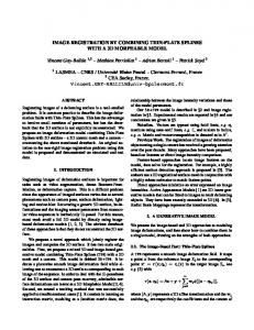
Figure 1: Registration results for images from boat (1,4) set.
4
EXPERIMENTS
In order to test our approach in Image Registration problems, a set of challenging sets of image pairs have been selected. They can be downloaded from Oxford’s Visual Geometry Group web page 2 . They present five types of changes between images in 8 different sets of images: Blur: bikes and tree sets, illumination: leuven set, jpg compresion: ubc set, zoom+rotation: bark and boat sets, and viewpoint: graf and wall sets. To check the accuracy of the registration, the normalized correlation coefficient (NCC) similarity measure has been calculated using the pixels of the overlapped area of both images. The NCC gives values from −1.0 (low similarity) to 1.0 (high similarity). The NCC is expressed as follows, with µ1 ,µ2 being the average of the gray level of both images and ℜ the overlapped area: ∑(xi ,yi )∈ℜ [(I1 − µ1 )(I2 − µ2 )] NCC(I1 , I2 ) = q ∑(xi ,yi )∈ℜ (I1 − µ1 )2 ∑(xi ,yi )∈ℜ (I2 − µ2 )2 (6) I1 and I2 have been introduced to simplify notation as: I1 = I1 (xi , yi ), I2 = I2 (xi0 , y0i ) We have focused on showing the results when solving challenging situations like the zoom+rotation and viewpoint sets of pair of images, particularly on boat, bark, graf and wall sets. The affine motion model has been used for images from sets bark and boat since there is not a viewpoint change. The main difficulty of this set is the presence of large rotations and changes of scale. The presence of moderate and large viewpoint changes forces to use the projective motion model instead of the affine one for images from graf and wall sets. Table 1 shows the average NCC calculated for the 2 http://www.robots.ox.ac.uk/ vgg/research/affine/index.html
Table 1: Average NCC obtained for each set.
After initial estimation After GLS estimation
bark 0.84 0.95
5
Figure 2: Registration results for images from graf (1,3) set.
experiments performed with the images belonging to each set, after initial estimation and after final GLS estimation. In general, the feature-based technique provides a good but not excellent (in terms of accuracy) initial estimation of the motion parameters, which are accurately improved after the GLS estimation. Figure 1 and 2 shows the results of the registration process obtained for some of the most difficult pairs from the four studied sets. The discontinuous white line mark the boundary of the reference image (i.e the first image of the pair). In general the proposed method is able to register all the images from bark and boat sets, but suffers in the case of strong viewpoint transformation, like in the case of registering the last images from wall and graf sets. For instance, when registering images 1 and 5 from graf set. The main problem in those cases is that, for the initial registration, there are not enough good feature point matches, due to the SIFT limitations to the presence of strong viewpoint changes. The registration of images from graf has an additional difficulty, the car changed its position between the image capture process (see the right-bottom corner of images). Therefore, the NCC obtained is not as good as the obtained for the other images (see Table 1) since those pixels are also been included in the calculation of the NCC. However, those pixels do not affect the accurate estimation of the motion parameters.
boat 0.81 0.91
graf 0.64 0.88
wall 0.85 0.92
CONCLUSIONS
In this paper an image registration approach has been presented. It uses a feature-based method, which allows to cope with large magnitude of changes in scale, rotation and viewpoint, combined with an accurate Generalized Least Squares motion estimation technique, which uses the result obtained by the feature-based method as initialization, and refines the estimation of the motion parameters. The proposed approach has been successfully tested using challenging real pairs of images with illumination changes, different blur level, different jpg compression, large changes of scale, large rotations and moderate viewpoint changes, obtaining high accuracy in the estimation of motion parameters. However, some problems arise in presence of very large viewpoint changes. This is due to the use of a nonviewpoint invariant interest point detector. As part of our future work we would introduce an viewpoint invariant point detector to overcome this shortcoming.
REFERENCES Brown, L. G. (1992). A survey of image registration techniques. ACM Computing Surveys, 24(4):325–376. Danuser, G. and Stricker, M. (1998). Parametric modelfitting: From inlier characterization to outlier detection. IEEE Transaction on Pattern Analysis and Machine Intelligence, 20(3):263–280. Lowe, D. G. (2004). Distinctive image features from scaleinvariant keypoints. International Journal of Computer Vision, 60(2):91–110. Mikolajczyk, K. and Schmid, C. (2004). Scale and affine invariant interest point detectors. International Journal of Computer Vision, 1(60):63–86. Mikolajczyk, K. and Schmid, C. (2005). A performance evaluation of local descriptors. IEEE Transactions on Pattern Analysis and Machine Intelligence, 27(10). Mikolajczyk, K., Tuytelaars, T., Schmid, C., and A. Zisserman, J. Matas, F. S. T. K. L. V. G. (2005). A comparison of affine region detectors. International Journal of Computer Vision, 65(1/2). Szeliski, R. (2004). Image alignment and stitching: A tutorial. Technical Report MSR-TR-2004-92, Microsoft Research.