Mar 5, 2002 - Nortel Networks Optical Components, 3500 Carling Avenue, Ottawa, Ontario, Canada K2H 8E9. M. Matus and J. V. Moloney. Arizona Center for ...
PHYSICAL REVIEW E, VOLUME 65, 036229
Achronal generalized synchronization in mutually coupled semiconductor lasers J. K. White Nortel Networks Optical Components, 3500 Carling Avenue, Ottawa, Ontario, Canada K2H 8E9
M. Matus and J. V. Moloney Arizona Center for Mathematical Sciences, The University of Arizona, Tucson, Arizona 85721 共Received: 22 October 2001; published 5 March 2002兲 Heil et al. 关Phys. Rev. Lett. 86, 795 共2001兲兴 recently discovered achronal synchronization of chaos in mutually coupled semiconductor lasers. This paper offers an analytic interpretation of their experiment using a simple rate equation model. Local eigenvalue analysis shows that isochronal synchronization is unstable; achronal synchronization, on the other hand, is stable if a generalized synchronization function is introduced. Single- and multimode simulations have substantiated this rate equation interpretation. Finally, there is a brief examination of ‘‘chaos pass filtering.’’ DOI: 10.1103/PhysRevE.65.036229
PACS number共s兲: 05.45.Xt, 42.55.Px, 42.65.Sf
Pecora and Carrol’s influential paper 关1兴 set in motion work synchronizing chaotic electronic 关2兴 and optical 关3兴 systems. Optical systems are especially interesting as they can have infinite-dimensional 关4,5兴 and spatiotemporal 关5,6兴 chaos. Most optical systems use a feedback delay ( 1 ) to drive the oscillator into a chaotic state and a coupling delay ( 2 ) to couple the light into another oscillator 关7兴. If 1 ⫽ 2 then achronal synchronization, where the driven oscillator’s dynamics lag or anticipate the driving oscillator’s dynamics, occurs 关8,9兴. Mutually coupled lasers, where each laser’s feedback is symmetrically replaced by the delayed electric field from the other, were not expected to have achronal synchronization since 1 ⫽ 2 . However, Heil et al. 关10兴 recently discovered achronal synchronization in mutually coupled lasers. Numerical models also possessed achronal synchronization 关10,11兴 but did not explain the lack of isochronal synchronization—that is, both lasers having the same dynamics at the same time. This paper offers an analytic interpretation of achronal synchronization in mutually coupled lasers. Isochronal synchronization can be described intuitively: each laser produces oscillations in its identical companion as if there were feedback with a time delay equal to the coupling delay. This solution is unstable. Achronal synchronization is stable, but it has a counter-intuitive construction: stable synchronization requires feedback with a delay time twice that of the coupling delay. This construction is an exact solution for only one laser, the other laser’s oscillations are not described by this solution and a small error determined by the constructed solution will always exist. Boccaletti, Pecora, and Pelaez’s framework for synchronization 关12兴 classifies systems with these characteristics as generalized synchronization instead of the simpler identical synchronization. The analysis begins with the standard single-mode rate equations for a semiconductor laser with delayed injection 关13兴 1063-651X/2002/65共3兲/036229共5兲/$20.00
de 1,2共 t 兲 ⫽⌫a 兵 关 n 1,2共 t 兲 ⫺n tr 兴 ⫺i ␣ n 1,2共 t 兲 其 dt ⫻e 1,2共 t 兲 ⫺ ␣ int e 1,2共 t 兲 ⫹ e 2,1共 t⫺ 兲 ,
n 1,2共 t 兲 dn 1,2共 t 兲 ⫽J⫺ ⫺a 关 n 1,2共 t 兲 ⫺n tr 兴 兩 e 1,2共 t 兲 兩 2 . dt n
共1兲
Here e 1,2(t) is the complex electric-field amplitude and n 1,2(t) is the carrier density for either the first or second laser. The usual rate equation coefficients are used: ⌫ is the confinement factor, a is the linear differential gain, n tr is the transparency carrier density, ␣ is the linewidth enhancement factor, ␣ int is the internal loss 共including the facet losses兲, J is the current pumping density, and n is the effective carrier lifetime. The coupling term consists of an attenuation and a delay . First, isochronal synchronization is shown to be unstable. e 1 (t)⫽e 2 (t)⫽e(t) exactly solves Eq. 共1兲 if e(t) is also the solution of an identical laser with feedback e(t⫺ ). This does not imply the existence of an external cavity but links, by analogy, the synchronized solution e(t) to the LangKobayashi solution 关13兴. Analogy between e(t) and external cavity lasers permits the use of established results, associates a physical interpretation to a mathematical abstraction, and generally illuminates the analysis. Small perturbations 共denoted by ␦兲 may drive the system from synchronization. Stability is governed by
65 036229-1
©2002 The American Physical Society
冉
J. K. WHITE, M. MATUS, AND J. V. MOLONEY
冉 冊
␦e ␦e* ⫽ ␦n
⫺
冊
PHYSICAL REVIEW E 65 036229
e 共 t⫺ 兲 共 1⫹e ⫺ 兲 e共 t 兲 ⫺*
0
⌫a 共 1⫺i ␣ 兲
0
⫺a 关 n 共 t 兲 ⫺n tr 兴 兩 e 共 t 兲 兩 2
e * 共 t⫺ 兲 共 1⫹e ⫺ 兲 e *共 t 兲
⌫a 共 1⫹i ␣ 兲 1 ⫺ ⫺a 兩 e 共 t 兲 兩 2 n
⫺a 关 n 共 t 兲 ⫺n tr 兴 兩 e 共 t 兲 兩 2
冉 冊
␦e ␦e* . ␦n
共2兲
The uncoupled case ( ⫽0) has solutions 0 ⫽0,
⫺ ⫾⫽
冋
册 冑冋
1 ⫹a 兩 e 共 t 兲 兩 2 ⫾ n
1 n
册
冋
y共t兲 t ⭐e ⫺ 兰 0 f 共 兲 d . y共0兲
共3兲
.
2
⫾ has a nonpositive real part providing that n(t)⫺n tr ⬎0. The time-averaged local eigenvalues determine stability: Theorem 1 Suppose dy/dt⫽A(t)y and A(t) is always diagonalizable. If every eigenvalue of A(t) satisfies Re()⭐⫺f(t) for some f (t)⬎0 then
冏 冏
2
⫹a 兩 e 共 t 兲 兩 2 ⫺8⌫a 2 关 n 共 t 兲 ⫺n tr 兴 兩 e 共 t 兲 兩 2
1 ⫹2
册
* e * 共 t⫺ 兲 关 ⌫a 2 共 1⫺i ␣ 兲关 n 共 t 兲 ⫺n tr 兴 兩 e 共 t 兲 兩 2 兴 e *共 t 兲
兩兩
冋
⫹ 1 ⫹2
e 共 t⫺ 兲 兩兩 e共 t 兲
册
⫻关 ⌫a 2 共 1⫹i ␣ 兲关 n 共 t 兲 ⫺n tr 兴 兩 e 共 t 兲 兩 2 兴 ⫽0.
共4兲
共5兲
Taking ⫽ 兩 兩 e i 0 and e(t)⫽A(t)e i (t) gives
This is not a rigorous stability criterion. Rigorous stability calculations are difficult, often tailored to a specific system 共see 关14兴 and references therein兲. Easier, nonrigorous methods can calculate stability without a loss of accuracy. One common method uses the Lyapunov exponents along a trajectory, with the system being stable if all Lyapunov exponents are negative 关1兴, but it does not relate stability along the many possible trajectories in a chaotic attractor. However, the eigenvalues of the Jacobian determine the Lyapunov exponents along a trajectory, so showing that the Jacobian has no positive eigenvalues is equivalent to showing that the Lyapunov exponents are negative 关15兴. This connection establishes local eigenvalue analysis as a credible, nonrigorous tool for evaluating synchronization stability. Although Corron 关16兴 found counterexamples to local eigenvalue stability analysis, he concluded that such stability analysis is still effective for most systems. All things considered, a system is unstable if a local eigenvalue is positive. Small values of r 兩 兩 共 r is the laser cavity round-trip time兲 perturb the eigenvalues from their ⫽0 values. This does not affect the stability of ⫾ but the marginally stable phase eigenvalue 0 is now either stable or unstable. Assuming the perturbation takes the form ⫽ 0 ⫹ r 兩 兩 1 ⫹ r2 兩 兩 2 2 ⫹¯ , where 0 ⫽0 and r 兩 兩 Ⰶ1, then to first order in r 兩 兩
1 ⫽⫺2
A 共 t⫺ 兲 冑1⫹ ␣ 2 A共 t 兲
⫻cos关 0 ⫹arctan ␣ ⫹ 共 t⫺ 兲 ⫺ 共 t 兲兴 .
共6兲
The delayed phase difference (t⫺ )⫺ (t) determines the isochronal synchronization stability. An upper bound on the delayed phase difference may be established by analogy between e(t) and the equivalent Lang-Kobayashi solution. In the Lang-Kobayashi system, the delayed phase difference determines the external cavity fixed points 关17兴 and their stability 关18兴. Specifically, near an equivalent unstable external cavity fixed point
冑1⫹ ␣ cos关 0 ⫹arctan ␣ ⫹ 共 t⫺ 兲 ⫺ 共 t 兲兴 ⬍⫺
1 . 兩兩 共7兲
e(t) approaches an unstable fixed point prior to an external cavity mode hop in the Lang-Kobayashi solution. As external cavity mode hops are a necessary condition for chaos in the Lang-Kobayashi system, Eq. 共6兲 inevitably becomes positive and isochronal synchronization turns unstable. On startup there will be an initial period of isochronal synchronization lasting until immediately after the first equivalent external cavity mode hop in e(t).
036229-2
ACHRONAL GENERALIZED SYNCHRONIZATION IN . . .
PHYSICAL REVIEW E 65 036229
feedback of e(t⫺ ) is a solution for neither subsystem. The equivalent Lang-Kobayashi solution requires a feedback term of e(t⫺2 ). Second, e(t) only satisfies the equation of motion for the subsystem e 2 ; e(t) is not an exact solution for the subsystem e 1 . Such a situation, where the synchronized solution solves one subsystem exactly but not the other, is best classified as generalized synchronization, which ‘‘associates the output of one system to a given function of the output of the other system’’ 关12兴. The linearized subsystems are of two different types: ␦ e 2 is homogeneous 共which determines stability兲 and ␦ e 1 is inhomogeneous 共which determines the generalized synchronization function兲. The homogeneous subsystem ␦ e 2 is
When isochronal synchronization loses stability a second solution may be chosen. Experiment and simulation suggest that achronal synchronization, consisting of a laggard solution e 1 (t)⫽ 关 1⫹ ␦ e 1 (t) 兴 e(t) and a leader solution e 2 (t) ⫽ 关 1⫹ ␦ e 2 (t⫹ ) 兴 e(t⫹ ), is selected. Direct substitution of the synchronous solution e(t) for e 1 (t) and e 2 (t) yields de 共 t 兲 ⫽⌫a 兵 关 n 共 t 兲 ⫺n tr 兴 ⫺i ␣ n 共 t 兲 其 e 共 t 兲 ⫺ ␣ int e 共 t 兲 dt ⫹
再
e共 t 兲
共 subsystem e 1 兲
e 共 t⫺2 兲
共 subsystem e 2 兲
共8兲
.
Two differences from isochronal synchronization are immediately obvious. First, a Lang-Kobayashi solution with
冉 冊
␦e2 ␦e* 2 ⫽ ␦n2
冉
冋
⫺ 1⫹
e 共 t⫺2 兲 e共 t 兲
册
冋
0 ⫺a 关 n 共 t 兲 ⫺n tr 兴 兩 e 共 t 兲 兩
2
e * 共 t⫺2 兲 ⫺ * 1⫹ e *共 t 兲
册
⫺a 关 n 共 t 兲 ⫺n tr 兴 兩 e 共 t 兲 兩
2
As before, for 兩 兩 ⫽0 Eq. 共3兲 governs the stability. The marginally stable eigenvalue 0 ⫽0 may become unstable for nonzero values of 兩 兩 . Using the previous eigenvalue expansion and solving for 1 gives the stability condition
冋
⌫a 共 1⫹i ␣ 兲 1 ⫺ ⫺a 兩 e 共 t 兲 兩 2 n
t
␦ D 共 t 兲 ⫽e 兰 t 0 D 共 兲 d
⫻
1 ⫽⫺2 冑1⫹ ␣ cos关 2 0 ⫹arctan ␣ 兴 2
⌫a 共 1⫺i ␣ 兲
0
册
A 共 t⫺2 兲 ⫹ cos关 2 0 ⫹arctan ␣ ⫹ 共 t⫺2 兲 ⫺ 共 t 兲兴 . A共 t 兲
冉 冉
t
t0
e ⫺ 兰 t 0 D 共 兲 d Q ⫺1 共 兲
冊
⫺ 1⫺
e 共 ⫺2 兲 e共 兲
⫺ * 1⫺
e * 共 ⫺2 兲 e *共 兲
冊
0
共9兲
冊
d
t
⫹ ␦ D共 t 0 兲 e 兰 t0D共 兲d t
⬅Q ⫺1 共 t 兲 † 关 e 共 t 兲兴 ⫹ ␦ e 1 共 t 0 兲 e 兰 t 0 共 兲 d ‡.
共10兲
This expression is identical to Eq. 共6兲 with the addition of a time-independent term cos关20 ⫹arctan ␣兴. The choice of arctan ␣’s branch guarantees that cos关20 ⫹arctan ␣兴 is greater than zero and furnishes a continually stabilizing force. As (t⫺2 )⫺ (t) is a chaotic variable with fluctuations greater than 2, 兰 t0 cos关(⫺2)⫺()兴d goes to zero for large times. Hence, the time-independent term dominates the stability for long times and achronal synchronization is stable. The inhomogeneous subsystem ␦ e 1 defines a generalized synchronization function
冉
冕
冊
冉 冊
␦e2 ␦ e *2 . ␦n2
共11兲
D is the diagonal matrix containing the local eigenvalues for the subsystem ␦ e 1 关Eqs. 共3兲 and 共6兲 with →2 兴, ␦ D is the state vector of the subsystem ␦ e 1 expressed in the basis of D, and Q is the change of coordinate matrix consisting of the local eigenvectors. 关 e(t) 兴 is the generalized synchronization function in the original basis. Both D and Q are timedependent matrices, making the exact calculation of the generalized synchronization function impractical 共if not impracticable兲. Numerical integration of Eq. 共1兲 has verified the interpretation presented here. Both lasers have been started from the same state and noise has driven them apart. This initializa-
036229-3
J. K. WHITE, M. MATUS, AND J. V. MOLONEY
PHYSICAL REVIEW E 65 036229
FIG. 2. Phase-space trajectory for the single-mode system. Equivalent stable 共unstable兲 external-cavity modes have been denoted as diamonds 共crosses兲. Up to 80 ns 共solid line兲 the trajectory had remained near the first stable external cavity mode. After 80 ns 共dashed line兲 the trajectory has jumped to the next stable external cavity mode and isochronal synchronization has become unstable.
FIG. 1. Startup of the mutually coupled single-mode system. Both lasers have been started from the same initial conditions and noise has continuously driven the system away from an identical state. 共a兲 Dashed line, eigenvalue 1 calculated for isochronal synchronization. Solid line, smoothed fit to 1 . Inset, enlarged view of the smoothed fit to 1 . 共b兲 Error function 兩 A 1 (t)⫺A 2 (t) 兩 . Dimensionless parameters: ⌫⫽1.1, a⫽1, n tr ⫽1, ␣ ⫽4, ␣ int ⫽0.27, J ⫽4.7⫻10⫺3 , n ⫽333.3, ⫽0.21⫻e i /4, and ⫽1515.15 共5 ns兲.
tion assured that the system began in the isochronal synchronization state. After the first external cavity mode hop, isochronal synchronization became unstable. When the instability occurs has been estimated from the error function 兩 A 1 (t)⫺A 2 (t) 兩 . For isochronal synchronization, the perturbation eigenvalue 1 and the error function are plotted in Fig. 1. Both have been averaged with a 2 full width at half maximum 共FWHM兲 Gaussian filter, which 共1兲 simulates a finite detector response, 共2兲 averages the inhomogeneous contribution from 关 e(t) 兴 , and 共3兲 satisfies the conditions for local eigenvalue stability analysis. For a delay of 5 ns, the effective bandwidth of the simulated detector is 100 MHz. Chaotic oscillations had set in by 40 ns, and the system was showing isochronal synchronization 共as measured by the error function兲 until 80 ns. Prior to 80 ns, 1 had some positive spikes but still had an overall negative value. At 80 ns 1 oscillates about 0, clearly violating the conditions for stability, and e(t) has had its first external cavity mode hop 共Fig.
FIG. 3. As in Fig. 1 but for the multimode system. 共a兲 Dashed line, eigenvalue 1 calculated for isochronal synchronization. Solid line, smoothed fit to 1 . Inset, enlarged view of the smoothed fit to 1 . 共b兲: Error function 兩 A 1 (t)⫺A 2 (t) 兩 . A many-body model 关11兴 with the same parameters as the single-mode model has been used.
036229-4
ACHRONAL GENERALIZED SYNCHRONIZATION IN . . .
PHYSICAL REVIEW E 65 036229
tions made to the laggard laser altered the leader laser’s response while periodic perturbations made to the leader laser did not disturb the laggard. The effect was labeled ‘‘chaos pass filtering’’ and from this the researchers concluded that achronal synchronization acted as a unidirectional coupled system: the leader laser was the driving subsystem and the laggard laser was the driven subsystem. In achronal synchronization, the difference between the two lasers is
2兲. After 80 ns achronal synchronization is stable and its associated eigenvalue is 1 ⫽⫺2 s⫺1 . This eigenvalue is larger than the isochronal eigenvalue (⬃10⫺8 s⫺1 ), is time independent, and is suitable for standard linear stability analysis. So, in a single-mode simulation, the external cavity modes have destabilized isochronal synchronization while achronal synchronization has not been affected. Mutually coupled lasers are not likely to run single mode, even if the solitary laser runs nominally single mode. Feedback 关19兴 and external injection 关20兴 excite multimode dynamics in single-mode lasers and multimode dynamics can change the synchronization stability 关5兴. Luckily, in many instances multimode systems conserve the single-mode structure, but such requires verification before affixing a single-mode interpretation to a potentially multimode system. Previous work established that achronal synchronization is stable for the multimode case 关11兴. The perturbation eigenvalue 1 and the error function 兩 A 1 (t)⫺A 2 (t) 兩 have also been calculated for the multimode system and are plotted in Fig. 3. Initially isochronal synchronization predominated but had lost stability within the first 100 ns, switching to achronal synchronization. As in the single-mode case the eigenvalue 1 had initially been negative, turning positive when isochronal synchronization lost stability. Unlike the singlemode situation, following the onset of chaos 1 had brief periods where it became positive, hampering isochronal synchronization. This relates to the increased difficulty of synchronizing infinite-dimensional spatiotemporal chaos, which is present in the multimode system 关5兴. Still the multimode laser has yielded to achronal synchronization by 80 ns and 1 has become positive 共the onset of the first power dropout drives 1 negative at 100 ns兲. Thus the single-mode interpretation applies to multimode systems as well. Finally, the interpretation developed here can shed light on a surprising result from 关10兴. In 关10兴, periodic perturba-
If the leader system is perturbed 关␦ e 1 (t 0 )⫽0 and ␦ e 2 (t 0 ) ⫽0兴, ␦ e(t) decays to 关 e(t) 兴 , achronal generalized synchronization is unaffected, and ‘‘chaos pass filtering’’ is observed. If the laggard system is perturbed 关␦ e 1 (t 0 )⫽0 and ␦ e 2 (t 0 )⫽0兴, achronal synchronization is affected and the system may be driven to a different solution such as observed in 关10兴. This paper has shown that, because of a phase instability, achronal synchronization is preferred over isochronal synchronization in mutually coupled lasers. Achronal synchronization requires a construction that results in the two lasers having different dynamics; viewed as such it is the first example of generalized synchronization in optical systems. Single- and multimode simulations explicitly show the phase instability’s onset. Finally, ‘‘chaos pass filtering’’ is understood as a natural consequence of achronal generalized synchronization.
关1兴 L. M. Pecora and T. L. Carroll, Phys. Rev. Lett. 64, 821 共1990兲. 关2兴 K. M. Cuomo and A. V. Oppenheim, Phys. Rev. Lett. 71, 65 共1993兲. 关3兴 R. Roy and K. S. Thornburg Jr., Phys. Rev. Lett. 72, 2009 共1994兲. 关4兴 H. D. I. Abarbanel and M. B. Kennel, Phys. Rev. Lett. 80, 3153 共1998兲. 关5兴 J. K. White and J. V. Moloney, Phys. Rev. A 59, 2422 共1999兲. 关6兴 J. Garcia-Ojalvo and R. Roy, Phys. Rev. Lett. 86, 5204 共2001兲. 关7兴 G. D. Van Wiggeren and R. Roy, Science 279, 1198 共1998兲; J.-P. Goedgebuer, L. Larger, and H. Porte, Phys. Rev. Lett. 80, 2249 共1998兲; I. Fischer, Y. Liu, and P. Davis, Phys. Rev. A 62, 011801 共2000兲. 关8兴 H. U. Voss, Phys. Rev. E 61, 5115 共2000兲. 关9兴 C. Masoller, Phys. Rev. Lett. 86, 2782 共2001兲.
关10兴 T. Heil et al., Phys. Rev. Lett. 86, 795 共2001兲. 关11兴 C. R. Mirasso et al., Phys. Rev. A 65, 013805 共2001兲. 关12兴 S. Boccaletti, L. M. Pecora, and A. Pelaez, Phys. Rev. E 63, 066219 共2001兲. 关13兴 R. Lang and K. Kobayashi, IEEE J. Quantum Electron. 16, 347 共1980兲. 关14兴 R. Brown and N. F. Rulkov, Chaos 7, 395 共1997兲. 关15兴 G. A. Johnson et al., Phys. Rev. Lett. 80, 3956 共1998兲. 关16兴 N. J. Corron, Phys. Rev. E 63, 055203 共2001兲. 关17兴 G. H. M. van Tartwijk, A. M. Levine, D. Lenstra, IEEE J. Sel. Top. Quantum Electron. 1, 466 共1995兲; I. Fischer et al., Phys. Rev. Lett. 76, 220 共1996兲. 关18兴 J. Mørk, M. Semkow, and B. Tromborg, Electron. Lett. 26, 609 共1990兲. 关19兴 G. Huyet et al., Phys. Rev. A 60, 1534 共1999兲. 关20兴 J. K. White et al., IEEE J. Quantum Electron. 34, 1469 共1998兲.
␦ e 共 t 兲 ⫽e 1 共 t 兲 ⫺e 2 共 t⫺ 兲 t
⫽e ⫺ 兰 t 0 共 兲 d ␦ e 1 共 t 0 兲 t
⫺e ⫺ 1 t e ⫺ 兰 t 0 共 兲 d ␦ e 2 共 t 0 兲 ⫺ 关 e 共 t 兲兴 t
⫽ 关 ␦ e 1 共 t 0 兲 ⫺e ⫺ 1 t ␦ e 2 共 t 0 兲兴 e ⫺ 兰 t 0 共 兲 d ⫺ 关 e 共 t 兲兴 . 共12兲
036229-5