Synchronization of Chaotic Systems with ... - APS Link Manager

PRL 96, 244102 (2006)

week ending 23 JUNE 2006

PHYSICAL REVIEW LETTERS

Synchronization of Chaotic Systems with Coexisting Attractors A. N. Pisarchik,1 R. Jaimes-Rea´tegui,2 J. R. Villalobos-Salazar,1,2 J. H. Garcıá-Lo´pez,2 and S. Boccaletti3 1

Centro de Investigaciones en Optica, Loma del Bosque 115, Lomas del Campestre, 37150 Leon, Guanajuato, Mexico 2 Universidad de Guadalajara, Centro Universitario de los Lagos, Enrique Dıáz de Leon, Paseos de la Montanã, 47460 Lagos de Moreno, Jalisco, Mexico 3 CNR - Istituto dei Sistemi Complessi, Via Madonna del Piano 10, 50019 Sesto Fiorentino (FI), Italy (Received 26 January 2006; published 21 June 2006) Synchronization of coupled oscillators exhibiting the coexistence of chaotic attractors is investigated, both numerically and experimentally. The route from the asynchronous motion to a completely synchronized state is characterized by the sequence of type-I and on-off intermittencies, intermittent phase synchronization, anticipated synchronization, and period-doubling phase synchronization. DOI: 10.1103/PhysRevLett.96.244102

PACS numbers: 05.45.Xt

The notion of synchronization provides a general approach to the understanding of the collective behavior of coupled dynamical systems and underlies a variety of modern techniques for chaos control and secure communications [1]. It is common to distinguish several types of synchronization, such as complete synchronization [2], generalized synchronization [3], phase synchronization [4], lag synchronization [5], and anticipated synchronization [6]. All these types of synchronization have been extensively studied in monostable chaotic systems (see, e.g., Ref. [7] and references therein). However, many dynamical systems exhibit multistability or coexistence of several attractors for a given set of parameters. Multistability was indeed observed in different fields of science, including electronics [8], lasers [9], mechanics [10], biology [11], nuclear physics [12], chemistry [13], and economy [14]. Multistable systems are extremely sensitive to perturbations due to their complexly interwoven basins of attraction. Synchronization of multistable systems still remains a long-standing and challenging problem of a broad interdisciplinary interest, both from the point of view of fundamental research and for practical applications. The prediction of bifurcations and synchronization are still largely debatable questions, even in such relatively simple systems as Ro¨ssler oscillators described by Caroll and Pecora [15]. The analysis is further complicated by the presence of chaos and fractal boundaries of basins of attraction of the coexisting attractors. For example, recently Guan et al. [16] studied synchronization of Lorenz and Ro¨ssler systems coupled in a drive-response configuration. They have found that the chaotic driving splits the synchronous attractor and thus generates bistability in the response system; both chaotic attractors were synchronized with the drive system. However, it is still unknown what happens with a state of a multistable system in the most general and therefore the most interesting case: when one multistable system is coupled with another identical multistable system. The answer to this question manifests inherent difficulties, when considering, e.g., two coupled chaotic bistable systems in a master-slave configuration. What hap0031-9007=06=96(24)=244102(4)

pens with the slave system when the coupling strength is increased? Intuitively, one might think that the slave system will first accommodate its state to the one of the master system and then the problem would reduce to the wellknown case of two identical chaotic monostable systems. However, this naı¨ve view is only partly true. In this Letter we demonstrate that the dynamics of coupled multistable systems is much richer and more complicated, including different types of synchronization, intermittency, shift of the natural oscillator frequency, and frequency locking. In order to illustrate our results, and without lack of generality, we consider two identical unidirectionally coupled piecewise linear Ro¨ssler-like electronic circuits [15,17,18]: dx1 x1 z1 y1 ; d dx2 x2 z2 y2 "y1 y2 ; d

dy2 x2 y2 "y1 y2 ; (2) d

dy1 x1 y1 ; d

dz1 gx1 z1 ; d where

(1)

(

dz2 gx2 z2 ; d

0; if x1;2 3 gx1 ;2 x1;2 3; if x1;2 > 3

(3)

)

is the piecewise linear function, t 104 s (t being the real time), 0:05, 0:5, 0:3, 15, and " 2 0; 1 is the coupling strength. All parameters are selected to reflect the real experiment that will be considered later. Equations (1)–(3) serve as a good model for many real systems including electronic circuits [2], chemical reactions [19], and biological systems [20]. Starting from different initial conditions the master and slave circuits stay without coupling (" 0) in different chaotic attractors with natural frequencies fm and fs . The coupling has no effect on the dynamics of the slave oscillator up to " 0:005 (0.5%) and the phase difference between the slave

244102-1

© 2006 The American Physical Society



PRL 96, 244102 (2006)

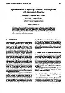
and master oscillations increases linearly with time. At a certain critical value of the coupling strength ("c "1 0:005 05), the slave system starts to switch intermittently between two coexisting chaotic attractors [Fig. 1(a)]. This is the weakest stage of synchronization. The phase of the master and slave oscillators can be defined as t ttk 2k 2 tk1 tk (tk being the time of kth maximum of the corresponding signal) [7]. Since within the windows where the slave and master oscillators stay in the same attractor the average time difference between successive peaks of the master and slave oscillations is equal to the natural period of the chaotic oscillations, we may approxis s m mate tm k1 tk tk1 tk 1=fm . Therefore, the phase difference between the peaks of the slave and master oscillations with the same number k can be written as s m 2tsk tm k fm (tk and tk being the times of kth maximum of the slave and master oscillations). As it can be seen in Figs. 1(b) and 1(c), within the windows drifts as a random walk in the range max min

2 (max and min being the maximum and minimum phase difference in the windows) featuring a normal probability distribution [Fig. 1(d)] and the most probable phase difference mod2 , i.e., the most probable synchronization state is the antiphase regime. While " is increasing, the jumps to the synchronization regime occur more frequently and decreases (Fig. 2). This means that the phases inside the windows become synchronized within a certain range of . We will refer to this regime as intermittent phase synchronization (IPS). IPS here implies intermittent switches between a phase synchronization state and an asynchronous state, at variance with other

phase intermittent phenomena observed in coupled map lattices [21]. The average anticipation time decreases with increasing " ( mod2 ! 0) while ! 0. The mean duration of the IPS windows (laminar phase), htL i, also decreases and finally at " 0:1 the windows of IPS disappear. A nontrivial result is that the oscillations of the slave system anticipate the oscillations of the master system and the maximum anticipation time is of the average period of the chaotic oscillations, 1=fm (Fig. 2). This means that the slave system is synchronized not with the present state of the master system but with its future state. Usually anticipated synchronization is observed in chaotic systems with time-delayed feedback [6,22]. However, as was mentioned by Voss [6] this phenomenon can also occur in continuous chaotic unidirectionally coupled systems without any delay. The origin of such a behavior is still an open problem which requires additional investigation. Here the anticipation process is confirmed by the fact that a maximum is emerging in the cross-correlation plot, and can be understood as the fact that a small coupling acts as a small change in initial conditions of the slave system, directing its phase trajectory to a future state of the master. In order to understand the transition route from asynchronous motion to perfect phase synchronization inside the IPS windows, we derive the type of intermittency by searching a scaling relation between htL i and ". With increasing ", htL i first decreases, then it increases, and finally it decreases again. It seems that the system has two saddle-node bifurcation points corresponding to largest htL i at "1 0:005 05 and "2 0:028. Near these critical points the power law htL i " "c p

(c)

(a)

∆φ (mod 2π)

y1, y2 (V)

is characterized by two different scaling exponents p 1=2 [Fig. 3(a)] and p 1 [3(b)]. The first scaling exponent is a characteristic of type-I intermittency associated with a saddle-node bifurcation [23]. The same scaling law was observed previously in a bistable chaotic system with external modulation [24,25]. The second critical exponent of 1 is a signature of on-off intermittency also associated with a saddle-node bifurcation. On-off intermittency was observed previously in many coupled chaotic

0

5

0

-5

−π

−2π -10 0.0

0.5

1.0

1.5

2.0

0

100 200 300 400 500 600

Time, t (s)

Peak number, k (d)

(b)

3 x10 10

Probability

0.15

∆φ

8 6 4

0.10

2π

0.05

δφ

0.5

1.0

Time, t (s)

1.5

2.0

0.00

−2π

−π

∆φ, δφ (mod 2π)

2 0 0.0

(4)

0

∆φ (mod 2π)

FIG. 1. Dynamics of the slave system at " 0:0051. (a) Time series demonstrating intermittent switches between coexisting attractors. (b) Temporal behavior of phase difference. increases linearly when the systems stay in different attractors and fluctuates around a certain value when the systems stay in the same attractor. (c) Random walk of phase difference inside window 1:33 s < t < 1:95 s where the systems stay in the same attractor. (d) Probability distribution of the phase difference inside the windows. The line is the Gaussian fit. The negative phase difference means anticipated synchronization.

π 0

-π ∆φ

-2π 0

1

2

3

4

5

6

7

8

9

ε (%)

FIG. 2. Average phase difference (filled dots) and fluctuation range (open dots) versus coupling strength inside windows of IPS. While " is increased, both the anticipation time and decrease leading to almost perfect IPS.

244102-2

4.5 4.0

4.5 4.0 3.5

3.5 3.0 -4.0

slope = -1.00+-0.05 error bars = 3%

5.0

log〈tL〉

5.0

log〈tL〉

(b)

slope = - 0.50+-0.02 error bars = 3%

-3.5

-3.0

-2.5

log(ε − ε1)

-2.0

3.0

-2.5

-2.0

-1.5

log(ε − ε2)

FIG. 3. Power law dependences of mean duration of IPS windows on coupling strength. The straight lines have slopes of (a) 1=2 and (b) 1 that characterize type-I and on-off intermittencies.

systems, including maps [26], Ro¨ssler oscillators [27], Duffing oscillators [28], and lasers [29]. The probability distributions of laminar phase versus the laminar length in the regions of type-I and on-off intermittencies are found to obey scaling laws with exponents 1=2 and 3=2, that also confirm these types of intermittency [26,30]. In the middle range of coupling, 0:01 < " < 0:028, the scaling exponent is positive; i.e., htL i increases with increasing ". We do not refer this regime to a particular type of intermittency, rather to a mixture of type-I and on-off intermittencies. Thus, the evolution of the bistable chaotic system from asynchronous behavior to perfect phase synchronization is realized through type-I and on-off intermittencies. One should expect type-I intermittency only for very weak coupling near the onset of intermittency "1 . The slave system is sensitive to only some high peaks of the master oscillations and does not feel other peaks. Therefore, the phase is not yet synchronized, i.e., analogously to the Brownian motion there exists the phase diffusion of inside the windows in a 2 phase interval ( 2) (see Fig. 2). In fact, in this range chaos of the master system acts as noise inducing type-I intermittency in the slave system [31]. Since only these high peaks force the slave system to change the attractor, the windows appear very rarely and their duration is large. With increasing ", the slave system becomes sensitive to more and more peaks of the master oscillations and hence the windows appear more frequently and their duration decreases. Finally, when " is increased so that the slave system is sensitive to all peaks of the master oscillations, the oscillations of the master system lock the oscillations of the slave system within a certain range of phase < 2. This occurs at the critical point "2 , the onset of on-off intermittency. From "2 the slave system becomes sensitive to the shape of the master oscillations that leads to phase synchronization. The transition from a phase-unlocked on-off intermittency to a phaselocked one was observed also in coupled chaotic identical monostable systems [32]. Thus, on-off intermittency (or modulational intermittency) results from chaotic driving of the slave system by the master oscillations. Besides IPS and anticipated synchronization another interesting phenomenon is observed in the coupled bistable

chaotic systems. At relatively strong coupling (" > 0:25) the fundamental frequency of the chaotic attractor of the slave system, fs , begins to decrease moving towards the period-doubling frequency of the master system, fm =2 (Fig. 4). As a result, slips of phase-synchronized perioddoubling oscillations arise. We will refer to this type of synchronization as period-doubling phase synchronization (PDPS). With a further increase in ", fs approaches fm =2 and the windows of PDPS becomes larger. Finally, fs becomes completely locked by fm =2 (at " > 0:5) and a stable PDPS regime is observed. Thus, the resonance interaction of the natural frequencies of the master and slave oscillators results in the frequency locking phenomenon in the form of phase-synchronized period-doubling oscillations (2:1 frequency locking). For " > 0:68, the 2:1 locking regime is interrupted by 1:1 frequency locking windows which appear more and more frequently with increasing ". At stronger coupling strengths, the amplitude of the perioddoubling oscillations decreases and the systems become completely synchronized at " > 0:7. The effects found in the numerical simulations are fully verified in experiments. We build two electronic circuits with parameters used in Eqs. (1)–(3) [2,18]. The experimental values of " at which PDPS and complete synchronization are observed are larger than those in simulations, because of experimental noise and a tolerance in values of electronic components. The latter fact makes the systems not completely identical to each other, which implies a stronger coupling to synchronize them. Although we do not get an exact quantitative coincidence, the qualitative agreement is evident. The route from asynchronous behavior to complete synchronization through anticipated synchronization in the windows of IPS [Fig. 5(a)], and PDPS [Fig. 5(b)] is clearly observed in the experiments, and confirmed by cross-correlation measurements. Previously anticipated synchronization was detected experimentally only in chaotic systems with time-delayed feedback [22]. The same scenario to complete synchronization is observed for different initial conditions of the master and slave systems. We also study synchronization in systems 0

fs

0.8 fs (kHz)

(a)

5.5



PRL 96, 244102 (2006)

0.7 0.6

fm/2

0.5

0.0 0.1 0.2 0.3 0.4 0.5 0.6 0.7 0.8 ε

FIG. 4. Dependence of natural frequency of slave system on coupling strength. fs is locked by the master oscillations and approaches fm =2. The solid line is the sigmoidal fit.

244102-3


PRL 96, 244102 (2006)

(b)

(a) 10

y1, y2 (V)

y1, y2 (V)

10 0

-10

0

-10 40

45

Time, t (ms)

50

65

70

75

80

Time, t (ms)

FIG. 5. Experimental time series demonstrated (a) anticipated synchronization within IPS window at " 0:07 and (b) perioddoubling phase synchronization at " 0:92. Master and slave oscillations are shown, respectively, by the dotted and solid lines.

with coexisting periodic and chaotic attractors and with two periodic attractors. In these cases synchronization dynamics is not as rich as in the case of coexisting chaotic attractors. Nevertheless, some features inherent to multistable systems remain, for example, IPS and PDPS are also observed in the system with coexisting periodic and chaotic attractors. In conclusion, we have studied, numerically and experimentally, synchronization of a bistable chaotic dynamical system coupled unidirectionally with another identical chaotic system. While the coupling strength is increasing, synchronization manifests itself, first, by intermittent jumps between two coexisting attractors demonstrating type-I and on-off intermittencies. Inside the windows where the systems stay in the same attractor, anticipated synchronization is observed. At the relatively strong coupling strengths, the interaction between fundamental frequencies of the coexisting attractors shifts the natural frequency of the slave oscillator towards a half of the natural frequency of the master oscillator, inducing phase-synchronized period-doubling oscillations. We argue that the phenomena described in this Letter are general for a wide class of multistable dynamical systems. Anticipated synchronization can be of interest for application in communication, because the slave system anticipates the state of the master system and hence one can get information about its future state. This work was supported by Consejo Nacional de Ciencia y Tecnologıá de Me´xico (Project No. 46973) and by the Italian Project MIUR-FIRB No. RBNE01CW3M001.

[1] A. Pikovsky, M. Rosenblum, and J. Kurths, Synchronization: A Universal Concept in Nonlinear Science (Cambridge University Press, New York, 2001). [2] L. M. Pecora and T. L. Carroll, Phys. Rev. Lett. 64, 821 (1990). [3] N. F. Rulkov, M. M. Sushchik, L. S. Tsimring, and H. D. I. Abarbanel, Phys. Rev. E 51, 980 (1995).


[4] M. G. Rosenblum, A. S. Pikovsky, and J. Kurths, Phys. Rev. Lett. 76, 1804 (1996). [5] M. G. Rosenblum, A. S. Pikovsky, and J. Kurths, Phys. Rev. Lett. 78, 4193 (1997). [6] H. U. Voss, Phys. Rev. E 61, 5115 (2000). [7] S. Boccaletti, J. Kurths, G. Osipov, D. L. Valladares, and C. Zhou, Phys. Rep. 366, 1 (2002). [8] J. Maurer and A. Libchaber, J. Phys. (Paris), Lett. 41, L515 (1980). [9] D. M. Heffernan, Phys. Lett. A 108, 413 (1985). [10] J. M. T. Thompson and H. B. Stewart, Nonlinear Dynamics and Chaos (Wiley, Chichester, 1986). [11] J.-F. Vibert, A. S. Foutz, D. Caille, and A. Hugelin, Brain Research 448, 403 (1988); A. Hunding and R. Engelhardt, J. Theor. Biol. 173, 401 (1995). [12] Tormod Riste and Kaare Otnes, Physica (Amsterdam) 137B+C, 141 (1986). [13] G. Jetschke, Phys. Lett. A 72, 265 (1979). [14] A. C.-L. Chian, E. L. Rempel, and C. Rogers, Chaos, Solitons & Fractals (to be published). [15] T. Carrol and L. Pecora, Nonlinear Dynamics in Circuits (World Scientific Publishing, Singapore, 1995). [16] S. Guan, C.-H. Lai, and G. W. Wei, Phys. Rev. E 71, 036209 (2005). [17] A. N. Pisarchik and R. Jaimes-Rea´tegui, J. Phys.: Conf. Ser. 23, 122 (2005). [18] J. H. Garcıá-Lo´pez, R. Jaimes-Rea´tegui, A. N. Pisarchik, C. Medina-Gutie´rrez, J. C. Jimeńez-Godinez, A. U. Murguıá-Hernandez, and R. Valdivia, J. Phys.: Conf. Ser. 23, 276 (2005). [19] A. Goryachev and R. Kapral, Phys. Rev. Lett. 76, 1619 (1996). [20] E. Mosekilde, Topics in Nonlinear Dynamics. Aplications to Physics, Biology, and Economics Systems (World Scientific, Singapore, 1996). [21] J. Y. Chen, K. W. Wong, H. Y. Zheng, and J. W. Shuai, Phys. Rev. E 64, 016212 (2001). [22] M. Ciszak, O. Calvo, C. Masoller, C. R. Mirasso, and R. Toral, Phys. Rev. Lett. 90, 204102 (2003). [23] P. Manneville and Y. Pomeau, Physica (Amsterdam) 1D, 219 (1980). [24] S. Boccaletti, E. Allaria, R. Meucci, and F. T. Arecchi, Phys. Rev. Lett. 89, 194101 (2002). [25] R. Meucci, E. Allaria, F. Salvadori, and F. T. Arecchi, Phys. Rev. Lett. 95, 184101 (2005). [26] J. F. Heagy, N. Platt, and S. M. Hammel, Phys. Rev. E 49, 1140 (1994). [27] M. Zhan, G. W. Wei, and C.-H. Lai, Phys. Rev. E 65, 036202 (2002). [28] R. J. Reategui and A. N. Pisarchik, Phys. Rev. E 69, 067203 (2004). [29] A. N. Pisarchik and V. J. Pinto-Robledo, Phys. Rev. E 66, 027203 (2002). [30] H. G. Schuster, Deterministic Chaos (VCH, New Yourk, 1989), 2nd ed. [31] H. Fujisaka, T. Yamada, G. Kinoshita, and T. Kino, Physica (Amsterdam) 205D, 41 (2005). [32] Meng Zhan, Gang Hu, D.-H. He, and W.-Q. Ma, Phys. Rev. E 64, 066203 (2001).

244102-4