ment that the algorithm based on the assumption that the number of people ... the
fig.2. The fig.2 shows that the sensor s1 reacted at the time step of 1, 3, ..... Seiichi
Honda, Ken-ichi Fukui , Koichi Moriyama, Satoshi Kurihara, Masayuki. Numao.
Acquisition of Sensor-Network Topology Based on Multi-Agent Pheromonal Coordination Hiroshi Tamaki1 , Ken-ichi Fukui2 , Masayuki Numao2 , and Satoshi Kurihara2 1
2
Department of Information and Physical Sciences, Graduate School of Information Science and Technology, Osaka University
[email protected] The Institute of Scientific and Industrial Research, Osaka University {fukui,numao,kurihara}@ai.sanken.osaka-u.ac.jp
Summary. To construct the ubiquitous network infrastructure, the sensor network technology is indispensable. And the information of the adjacent relation of each sensor is very important especially for the sensor network, but getting this information by an automatic way without a help by human is a hard work. So, in this paper, we will propose a new methodology of constructing the adjacent relation of sensor network using ant colony optimization algorithm. This methodology can extract automatically the adjacent relation without using prepared sensor location information and RFIDs to identify the each human. We implemented the prototype system, and verified the basic effectiveness of the system by using the simulation and the experiment using the real data.
1 Introduction Recently, study of the ubiquitous computing and/or ubiquitous network systems is very attractive along with the rapid development of the information and communications technology[2]. In the ubiquitous network systems, all kind of information devices such as computer, cellular phone, electrical appliance, medical equipment, and various sensors will be connected each other. So, anyone will be able to make use of any kind of information without stress, anywhere, anytime. To construct the ubiquitous network systems, we need to bring into reality the idea of ”context-awareness” as an essential element[8]. ”Context” refers to the situation in which ubiquitous network devices are embedded, and ”awareness” refers to the recognition of ”context” with ubiquitous network. One goal of context awareness is to acquire and utilize information about the context to provide services that are appropriate to the particular people, place, time, events, etc. And, the ubiquitous network systems is expected to implement
2
Hiroshi Tamaki et al. 3
2
2 1
3
4
4
5
1
A sensor network
5
Adjacent relationships
Fig. 1. Example of adjacent relationships of a sensor network
the context-awareness by using the sensor network, which is made up of many sensors. To extract human motion in a sensor network system, the information of adjacent relationships among sensors is necessary[7]. The adjacent relationships indicates physical connectivity among sensors from the point of view of a person’s movement in a sensor network(fig.1). Usually, this information is given to the system by hand[3]. However, to investigate and input the information of sensor topology becomes so hard in proportion to the scale of the sensor network system. In addition, once a structure of the network changes, for example by adding/removal of the sensor unit and by rearrangement of the network etc., we have to reinvestigate adjacent relationships again by hand. To repeat the investigation and input over again and again is troublesome work, and raise the possibility of making a mistake. Especially, in an emergency situation, there is no room to investigate the modified topology. So, it is necessary for the sensor network system to be able to acquire its own structure automatically without any previous knowledge. In a study of D.Marinakis et al., they constructed the adjacent relationship of a sensor network and traffic pattern of persons in the network using stochastic expectation maximization[4]. They succeeded in constructing the flexible algorithm dependent on no previous knowledge but the information of observed data by each sensor. But, the performance of their algorithm so deeply depends on the number and traffic pattern of persons in the environment that the algorithm based on the assumption that the number of people in the network and the traffic pattern is constant. Moreover, this algorithm needs many analyses with a variety of an estimated number of person and traffic pattern to acquire the number of person. It takes so much time that this algorithm is said to be far from practical use. In this paper, we will propose and verify the algorithm predicting the sensor relationships using only the sensor data. To propose the algorithm, at least it must include the following three capabilities: (1) Anytime characteristic - the algorithm should be able to output the result as good as possible through analysis on finite time even if the scale of network become larger or the frequency of movement in the network gets higher. (2) Adaptability - the algorithm don’t have to require special tuning for any types of environments. Also, the algorithm should adapt a change of network structure automatically. (3) Robustness - the algorithm should keep high accuracy of analysis result
Acquisition of Network Topology Based on Pheromonal Coordination
3
even though a ratio of noise data caused by moving of multi persons at the same moment or sensing errors of sensors increase. Meanwhile, the Ant Colony Optimization (ACO) algorithm, which is a one of the most famous pheromone communication model deriving from the swarm behavior of nature ants[5]. ACO is well known as having so strong robustness and adaptability for the dynamic changes of the environment, and various kinds of optimization problems has been solved by ACO based approaches[1][6]. The ability of ACO is very attractive for our needs, so we constructed the algorithm based on ACO. The rest of this paper is organized as follows. The section 2 shows the outline of the proposed algorithm. And the section 3 describes the details of it. In the section 4 and 5, we show the experimental result using artifice sensor data and actual one. In the section 6, we describes the conclusion of this study.
2 Pheromone Communication Algorithm 2.1 Estimation of Standard Traveling Time between Sensors In the proposed algorithm, we use following sensor reaction data as shown in the fig.2. The fig.2 shows that the sensor s1 reacted at the time step of 1, 3, and 7 the sensor s2 reacted at the time step of 2, 3, 5, and 8. The reaction data of sensor n
On = {t n1 , t n2 , t n3 ・・・} , The time stamps when sensor n reacted
(Data example )
O1 = { 1, 3,
7,
2
O = { 2,3,
・ ・ ・
5,
・・・}
8, ・・・}
Fig. 2. The format of sensor reaction data
If sensor si and sensor sj are set to be adjacent, it can be thought that the traveling time between two sensors of each person becomes roughly the same. So, when the sensor si reacts at timestept1 and the sensor sj reacts at timestept2 , and |mi,j − (t2 − t1 )|, in which mi,j is an average traveling time between si and sj , becomes so small, we can think that these two sensors reacted by the travel of one person from si to sj . To the contrary, when |mi,j −(t2 −t1 )| becomes so big, it can be though that these two sensors reacted by different two persons. Therefore, if mi,j is calculated from very long sensor reaction data log and the |mi,j − (t2 − t1 )| usually becomes so small, we can think that si and sj are placed to be adjacent even if we preliminarily do not 1 know the relation of both sensors. At this point, we define ωi,j = |mi,j −(t 2 −t1 )| as adjacent likelihood of that the sensor si and sj are placed to be adjacent.
4
Hiroshi Tamaki et al.
But, the methodology for estimation of a adjacent relation of two sensors by using ω has several weak points. For example, even when different persons make reactions of each sensor simultaneously and the interval time becomes near to the standard traveling time of them, we make a misunderstanding that is we think both sensors are placed to be adjacent. Moreover, of course, it is necessary to think about noise like mis-reaction of sensor, and it is also important to think about dynamical change of adjacent relation of sensors (for example, we occasionally re-arrange furniture of our office and room). 2.2 Necessary Functions To solve the above problems, the following functions are effective. 1.Positive feedback loop Positive feedback loop is necessary to accelerate a process in which such the two sensors having the higher adjacent likelihood can be given the higher ω. 2.Avoidance of local solutions It is necessary to avoid such a mis-detection that two sensors cannot be considered like they are in the adjacent relation, due to extreme bias of adjacent likelihood. The above “item 1” and this “item 2” are in the relation of the trade-off. 3.Using other criteria to calculate the adjacent likelihood Not only using interval time of sensor reaction which is the basic methodology to consider that two sensors are in the adjacent relation, but also using other criteria is necessary to improve accuracy and convergence. 4.Deletion of old information To adapt to dynamic change of the environment, it is necessary to delete relatively old information of sensor reaction data log. Although these items are all effective, it is difficult to coordinate them by hand, due to the existence of trade-off between them. So, in this paper we will propose a new methodology to calculate the adjacent likelihood of sensors based on ACO (Ant Colony Optimization which is one of pheromone communication models). In the proposed methodology, all the items are implemented and adjustments between them are autonomously done. In our methodology adjacent likelihood is considered as amount of pheromone, and the pheromone is accumulated by using both adjacent likelihood calculated from passed sensor reaction data and presumption distance between sensors derived from standard traveling time. By the accumulation mechanism, the positive feedback loop in which the adjacent likelihood entirely increase is formed in the sensors of being placed at adjacent relation. To the contrary, in the sensors of being placed at non-adjacent relation, the noise deletion due to simultaneous sensor reaction by several persons can be done. Moreover, since the pheromone gradually evaporates old information is automatically
Acquisition of Network Topology Based on Pheromonal Coordination
5
removed. This means that new information is always given priority. As for the coordination of the items, it is autonomously and indirectly controlled by the interaction of agents using pheromone. 2.3 Virtual Graph The proposed methodology using pheromone communication model is executed on a following virtual graph G on which agents move between sensors and the pheromone interaction happens. G = (V, E) is a virtual directed graph and each node vi ∈ V corresponds to each sensor si ∈ S in the real environment. Edge ei,j ∈ E means the edge from the node vi to the vj . Before starting calculation, there is no information about the adjacent relation, so G is complete graph initially. Accumulation and deletion of several kinds of pheromone are done on each ei,j , and we propose the following three kinds of them:τ , ω, and ϵ •
•
•
Pheromone concerned to adjacent likelihood ω (hereinafter ”edge pheromone”) In the proposed methodology, the whole sensor reaction data is divided into several data units(mentioned in the next section), and the calculation is done for each unit repeatedly. And ω shows the adjacent likelihood of each unit. ω is always initialized before the calculation of each data unit. Pheromone being output by agents ϵ (hereinafter ”agent pheromone”) Each agent outputs ϵ corresponding to ω on each edge as evaluated result of the edge. ϵ is always initialized before the calculation of each data unit too. Pheromone distribution data set τ (hereinafter ”pheromone distribution”) τ shows the accumulation of each ϵ, that is τ shows the total adjacent likelihood of reflecting the calculation result of all units. τ is updated whenever the calculation for a new unit has finished.
Initially, τ (0) (in this paper, τ (0) = 300) is assigned for the whole edges. As for the agents, a agents move on the G and they output the pheromone, depending on the amount of the pheromone on each edge. Initially, they are placed on the G homogeneously. 2.4 Detail of the Calculation The whole sensor reaction data is divided into the several data units Ot containing the data of the interval of time T as shown in the fig.3. The standard traveling time m and the pheromone distribution τ are updated whenever the calculation for each data unit has finished. And whenever the calculation for each data unit has finished, it is judged whether two sensors are adjacent for the whole sensors. Then location of each agent, and ω and ϵ are initialized for the calculation of the next data unit. The calculation for the next data unit is executed using m and τ updated in the previous process. The fig.4 shows the whole sequence of the algorithm.
6
Hiroshi Tamaki et al. Sensor reaction data
O1 = {1,3,8・・・ ,9826,10003,10005, ・・・,19580,20031,20045 ・・・} O2 = {2,3, ・・・,9561,9765,10011, ・・・ 18120,20003, 20021
T
T
T
Data unit O 1 O1 1 = {1,3,8 ・・・ ,9826}
O
O2 1 = {2,3 ・・・ 9561,9765}
O2 2 = {10011,
Data unit O3
Data unit O2 1
・・・}
= {10003,10005, ・・・ ,19580}
2
・・・
,18120}
Fig. 3. Example of the data unit of T = 10, 000. Start Process
(h) Initialization of the environment
Effect
Input data unit Ot
Pheromone Generation Phase
(a) Update standard time distance (b) Generate edge pheromone Agents Movement Phase
(c) Move Agents (d) Add agent pheromone
Pheromone Evaporation Phase
(e) Evaporate pheromone distribution (f) Update pheromone distribution
(g) Criterion for adjacent relation exist Ot+1?
Output adjacent relationship
Yes
No
End
Utilize previous results
Fig. 4. Overview of the proposed algorithm
3 Adjacent Relation Acquisition Algorithm In this section, the algorithm and adjacent relation determination are described in detail. 3.1 Pheromone Generation Phase This phase updates M (t) 3
3
from Ot and generates ω(t) onto the graph.
M (t) equals set of standard traveling time m(t)i,j M (t) = {m(t)i,j |∀i, j, i ̸= j}.
Acquisition of Network Topology Based on Pheromonal Coordination
7
(a)Update standard traveling time M First of all, a frequency distribution di,j (t) of time distance is created from Ot . dci,j (t) represents a frequency that a time interval between two sensors si and sj is equal to c within Ot . After updating an accumulated frequency distribution Di,j (t) using the current di,j (t) (eq.(1)), update a standard traveling time M (t) using Di,j (t) (eq.(2)). Since Di,j (t) is an accumulation of time distance di,j (t) of each data unit, M (t) is the most frequent time distance up to now. c c (t) = Di,j (t − 1) + dci,j (t). Di,j c mi,j (t) = arg max Di,j (t). 1≤c≤50
(1) (2)
(b)Generate edge pheromone ω c ωi,j (t) is represented by sum of an adjacent likelihood ∆ωi,j (t) that each time interval c has (eq.(3),(4)).
dci,j (t) . |mi,j (t) − c| c (t). ωi,j (t) = Σc ∆ωi,j
c (t) = ∆ωi,j
(3) (4)
3.2 Agent Movement Phase In this phase, each agent moves based on τ (t) and M (t), and adds ϵ(t) onto an edge based on ω(t). (c)Move agents Each agent moves only once on an edge within an agents movement phase, and can move to any node except the current position. Each agent selects a route based on the previous searching result τ (t) and heuristics η(t). ηi,j (t) is an inverse of mi,j (t) of its route. The less mi,j (t) is, i.e., the shorter distance between sensors is, the larger value is . Each agent is set to prefer an edge on which a lot of τ (t) remains. Therefore, it can focus search on the edges that have high adjacent likelihood by previous search. Also, since an agent is set up to prefer a route that has high η(t), it can search more effectively. It is high possibility that adjacent sensors are located near compared to non-adjacent sensors. A probability pki,j (t) that an agent k moves from vi to vj in Ot is given by: [τi,j (t)][ηi,j (t)]γ . γ j,j̸=i [τi,j (t)][ηi,j (t)]
paki,j (t) = ∑
(5)
8
Hiroshi Tamaki et al.
γ is a weight for τ (t), it gives priority to the information for each agent. In addition, each agent is set up to select a route randomly with constant probability r not depending on τ (t). This prevents the obtained adjacent relation from falling into the local solution. The local solution might be obtained by the effect of feedback loop of a pheromone increase. γ = 1 and r = 0.1 are used in this paper. (d)Add agent pheromone ϵ After movement, each agent discharges an agent pheromone ∆ϵki,j (t) onto its edge as the evaluation value of the route. The evaluation value reflects the information of Ot using ωi,j (t) that is generated in Pheromone Generation Phase. Eq.(6) represents the agent pheromone ∆ϵki,j (t) that the agent k who passed ei,j add onto ei,j . Also eq.(7) represents the amount of agent pheromone ϵi,j (t), where n is the number of agents who move ei,j . ∆ϵki,j (t) = ωi,j (t). n ∑ ∆ϵki,j (t). ϵ′i,j (t) = { ϵi,j (t) = z
(6) (7)
k=1
( )ϵ′ (t) } 1 i,j 1− 1− z
(8)
Eq.(8) prevents strong bias of the pheromone distribution. When sum of agent pheromone ϵ′i,j (t) that the agents who moved ei,j discharge is low, the pheromone amount proportional to that value is added. However, contribution by the increase of the agent pheromone decreases with increasing ϵ′i,j (t). z is set to 1,000 in this paper. 3.3 Pheromone Evaporation Phase This phase evaporates τ (t) and updates τ (t) using ϵ(t). (e)Evaporate pheromone distribution τ τi,j (t) that is on each edge decreases by the evaporation rate ρ every evaporation phase. Eq.(9) gives the evaporation calculation: ′ τi,j (t) = (1 − ρ)τi,j (t).
(9)
Acquisition of Network Topology Based on Pheromonal Coordination
9
(f )Update pheromone distribution τ ′ After evaporating, τi,j (t) is updated by being combined with ϵi,j (t) that is generated in the Agent Movement Phase. Eq.(10) gives the update formula for τi,j (t) in Ot : ′ τi,j (t + 1) = τi,j (t) + ϵi,j (t).
(10)
In this way, later searching information is reflected in a constant ratio by discarding old searching information. The evaporation rate ρ affects an update speed. The smaller ρ is, the more weight to later information is. ρ = 0.01 is used in this paper. In general, when ρ is small, a stable solution can be obtained, however, a convergence speed is slow. Meanwhile, when ρ is large, a convergence speed is fast, however, an unstable solution may be obtained depending on each data unit. 3.4 Determination of Adjacent Relation This section describes the determination of adjacent relation after finishing an analysis for Ot and the initialization of G for Ot+1 . (g)Criterion for adjacent relation τ (t) represents a adjacent likelihood as a result of total analysis up to now. An edge is determined as an adjacent relation when τ (t) is greater than certain threshold. The threshold is given by α times the average of all pheromone distribution τ (t) as shown in eq.(11). α is set to 0.8 in this paper. Here, |V | is the number of nodes. threshold (t) = α ×
Σi,j τi,j (t) . |V |2
(11)
(h)Initialization of the environment If the next data unit Ot+1 exists after finishing above phases, it restarts analysis from the pheromone generation phase using Ot+1 after initializing the environment. As for an initialization, ω(t) and ϵ(t) are discarded, also the agents are allocated evenly onto each node. Only τ (t + 1), M (t), and D(t) are inherited to the next analysis.
4 Empirical Verification using Simulation For the sake of checking the basic effectiveness of the proposed algorithm, we conducted verification experiments by simulation. In this section, we show the result of experiment using artificial sensor data. First, we developed a tool for analysis as shown in the fig. 5.
10
Hiroshi Tamaki et al.
Adjacent Relationships
Fig. 5. The interface of analysis tool.
4.1 Preparation of The Data for Simulation We prepared the sensor reaction data for simulation by the virtual sensor network environment(fig.6. This virtual environment is built up with staff rooms and aisles attached sensors to, and in which staffs move around. Each staff is set to repeat moving from one room to another randomly and asynchronously. At every time step, each staff decides whether to begin moving or not respectively according to a probability ”movement frequency”, which represents how often staffs start to move. When a staff passes ahead of one sensor, the sensed data from this sensor is sent and stored with the time stamp of the sensed time. A mis-detection of sensor is also happened, which occurs depending on a probability ”mis-reaction frequency”. Whenever time T passes, the data unit Ot is created and the analysis is performed.
17 14
11
19
16
9
13
8 18
15
12
10
n
7 4
Sensor n
6
5 0
2 1 3
Staff
Fig. 6. Virtual sensor network environment E2 .
Acquisition of Network Topology Based on Pheromonal Coordination
11
In this experiment, we prepared two patterns of virtual environment, E1 and E2 , which has 10 and 20 sensors, and also has 6 and 14 staffs. Movement frequency was also set up for three patterns FLow , FN ormal and FHigh , and mis-reaction frequency was also set up for M0 , M20 and M50 4 . By choosing these elements, we built a variety of virtual sensor networks. As for the algorithm parameter a and T , we used the following values depending on simulation elements E and F . ({E, a} = {E1 , 2, 000},{E2 , 4, 000}}, {F, T } = {FLow , 15, 000},{FN ormal , 8, 000},{FHigh , 1, 000}) 4.2 Verification about Robustness First, we verified the robustness against noise data. We divided noise data into two types: one is caused by multi-walkers movements and another by mis-reaction of a sensor. We controlled these noise probabilities by selecting simulation elements E, F , M . For comparison, we constructed two more adjacent likelihood calculation algorithms Test1 and Test2. In the Test1, adjacent relations are judged from the adjacent likelihood ω without being weighed at all. Test2 is based on Test1 and only adopt the information of η to weigh ω. We tested the robustness with the noise production probability related with the ratio of the multi-persons simultaneous movements varied. Six kinds of virtual environment was prepared by pairing E with F (M20 is used), and for each environment we performed the calculation for 1,000,000 time steps using the proposed algorithm, Test1 and Test2. Each of the calculation was repeated for ten times and of which the average of accuracies was calculated (accuracy is the ratio of correct adjacent relationships acquired by calculation). The mean value of accuracies is shown in fig.7, and the process of acquisition of adjacent relationships by the proposed algorithm is shown in fig.8. Virtual Environment E 1
Virtual Environment E 2 100
100
90
Accuracy (% )
Accuracy (%)
90 80 70 60
Proposed Algorithm Test1 Test2
FNormal Movement Frequency
70
60
50
FLow
80
FHigh
50
Proposed Algorithm Test1 Test2
FLow
FNormal Movement Frequency
FHigh
Fig. 7. Relationship between F and accuracy.
Next, the verification about the robustness against mis-reaction noise of sensor was performed. We prepared six pattern environments by pairing E 4
Mx means that each sensor fails to detect at the probability of x%
12
Hiroshi Tamaki et al. Adjacent Relationships
Adjacent Relationships
Initial pheromone distribution
After the 300,000 time steps Adjacent Relationships
Adjacent Relationships
After the 50,000 time steps
After the 500,000 time steps
Adjacent Relationships
Adjacent Relationships
After the 100,000 time steps
After the 1,000,000 time steps
Fig. 8. The transition of acquiring adjacent relationships.
with M (FN ormal is used), and experimented in the same way as the environments using multi-persons simultaneous movements noise. Fig.9 shows the result. Virtual Environment E 2
Virtual Environment E 1
90
Accuracy (% )
100
90
Accuracy (% )
100
80 70 60
Proposed Algorithm Test1 Test2
M20 Mis- reaction Frequency
70 60
50
M0
80
M50
50
Proposed Algorithm Test1 Test2
M0
M20
M50
Mis- reaction Frequency
Fig. 9. Relationship between M and accuracy.
Fig.7 and fig.9 represent that the proposed algorithm has superiority over comparison algorithms in the analysis accuracy. In addition, sensor data which our algorithm needed to attain 90% of accuracy was always fewer than other algorithm. So, we concluded that the proposed algorithm has robustness against noise data.
Acquisition of Network Topology Based on Pheromonal Coordination
13
4.3 Verification about Adaptability Second, we verified the adaptability against the dynamic change of the topology of sensor network systems. Structure change is generated by raising a failure of one sensor and a replacement of two sensors. E1 , FN ormal , M20 were selected for the simulation elements, and after 500,000 time steps passed network structure was shifted. A time to recover the accuracy up to 90% was taken as a barometer of adaptability to a structure change. Fig.10 shows the process of adaptation to a dynamic change of network structure. Adjacent Relationships
Adjacent Relationships
After the 500,000 time steps (Before the structure change) Adjacent Relationships
After the 1,400,000 time steps Adjacent Relationships
After the 700,000 time steps
After the 2,000,000 time steps
Fig. 10. The process of adaptation.
As a result, the proposed algorithm needed about half time to recover as much as the algorithm not using pheromone communication system. Therefore, we conclude that the proposed algorithm has basic adaptability to a environment change.
5 Empirical Verification using Real World Sensor Data This section describes the empirical verification using the real world sensor data. We used the sensor reaction data that were obtained from the infrared sensor network installed in our laboratory. A person presence detection is done by reading a reflection intensity from an sensor that beams infrared laser from itself. The data was collected 30 days with 31 infrared sensors that are installed in the three rooms. The proposed algorithm is compared with the Test1 and Test2 that were used in section 4. Fig.11 shows the layout of the sensor network. The sensor data was collected 24 hours, and the average of the number of reaction in each sensor was 2143.2. Also the structure of the network did
14
Hiroshi Tamaki et al.
Sensor Fig. 11. Actual layout of the sensor network.
not change during the period. The parameter T = 10, 000 and a = 20, 000 are used. Fig.12 shows the result by the proposed algorithm, Test1 and Test2.
Proposed Algorithm
Accuracy (% )
Test2 Test1
000
Time Step
Fig. 12. Analysis accuracy by the algorithms using the real world data and obtained adjacent relationships.
Fig.12 shows that the proposed method is superior to the test algorithms. (Accuracy: Proposed· · ·87%, Test1· · ·53%, Test2· · ·64%) Note that it keeps stably high accuracy after around 300,000 time steps. Each data unit is created and analyzed by every one and half hour when converted into real world’s time. It can be considered that there are large difference in amount of sensor reaction information between daytime and night or holiday. Moreover, when a person makes only one sensor react during his one movement episode, this case becomes a noise in addition to the multi-person movements and sensor miss-reaction, because it is impossible to extract a sensor reaction relation when only one sensor reacts. Since the proposed algorithm assumes that sensor reaction information is sequence of person’s movement, a single sensor reaction hinders accuracy improvement. However, the proposed method also shows robustness for this problem compared to the test algorithm.
Acquisition of Network Topology Based on Pheromonal Coordination
15
6 Conclusion From the evaluation by the simulation and the verification experiment in the real world, basic effectiveness of the proposed methodology could be verified. As for the real environment experiment, that is our laboratory, 15 persons are working. But the number of people at work is different depending on a day of the week and time. Habitual behavior of each person is of course different and has own week and day schedules. Our proposed methodology based on the pheromone communication model can adapt to these diversity of persons, but unfortunately it might be difficult in the methodology of D.Marinakis. So, the proposed methodology has the following features: (1) Positive feedback loop is used to accelerate a process in which such the two sensors having the higher adjacent likelihood can be given the higher likelihood in autocatalytic way. (2) When each agent selects the node to move, a random selection is done at a constant rate. This mechanism, that is heterogeneous factor, is very effective. (3) Not only using interval time of sensor reaction which is the basic methodology to consider that two sensors are in the adjacent relation, but also using other criteria, that is the standard traveling time, is very effective to improve accuracy and convergence. (4) Since the pheromone gradually evaporates, old information is automatically removed, that is, new information is always given priority. These features support all of the necessary functions in the section 2, and show the effectiveness of the pheromone communication model.
References 1. Ajith Abraham and Vitorino Ramos,Web Usage Mining Using Artificial Ant Colony Clustering and Linear Genetic Programming ,CEC 03,2003 2. S. Kurihara, S. Aoyagi, T. Takada, T. Hirotsu and T. Sugawara, AgentBased Human-Environment Interaction Framework for Ubiquitous Environment, INSS2005, 2005. 3. Seiichi Honda, Ken-ichi Fukui , Koichi Moriyama, Satoshi Kurihara, Masayuki Numao. Extracting Human Behaviors with Infrared Sensor Network, Fourth International Conference on Networked Sensing Systems (INSS) 2007, 2007 4. Dimitri Marinakis and Gregory Dudek, Topological Mapping through Distributed Passive Sensors, IJCAI-07, 2007. 5. Marco Dorigo and Gianni Di Caro, The Ant Colony Optimization MetaHeuristic, New ideas in optimization, 1999. 6. John A Sauter,Rbert Matthews,H Van Dyke Parunak and Sven A Brueckner, Performance of Digital Pheromones for Swarming Vehicle Control ,Proceedings of the fourth international joint conference on Autonomous agents and multiagent systems, 2005 7. Taisuke Hosokawa and Mineichi Kubo, Person tracking with infrared sensors, Proceeding of the KES2005, pp 682–688, 2005. 8. Thomas P. Moran and Paul Dourish, Context-Aware Computing ,Special Issue of Human-Computer Interaction, Volume 16, 2001