{ting,nick,paul,jake,marni,movellan}@mplab.ucsd.edu. AbstractâWe explore how CERT [15], a computer expression recognition toolbox trained on a large ...
Action Unit Recognition Transfer Across Datasets Tingfan Wu, Nicholas J. Butko, Paul Ruvolo, Jacob Whitehill, Marian S. Bartlett, Javier R. Movellan Machine Perception Laboratory, University of California San Diego {ting,nick,paul,jake,marni,movellan}@mplab.ucsd.edu
Abstract—We explore how CERT [15], a computer expression recognition toolbox trained on a large dataset of spontaneous facial expressions (FFD07), generalizes to a new, previously unseen dataset (FERA). The experiment was unique in that the authors had no access to the test labels, which were guarded as part of the FERA challenge. We show that without any training or special adaptation to the new database, CERT performs better than a baseline method trained exclusively on that database. Best results are achieved by retraining CERT with a combination of old and new data. We also found that the FERA dataset may be too small and idiosyncratic to generalize to other datasets. Training on FERA alone produced good results on FERA but very poor results on FFD07. We reflect on the importance of challenges like this for the future of the field, and discuss suggestions for standardization of future challenges.
I. I NTRODUCTION Thanks to the use of machine learning methods, the field of automated facial expression recognition is rapidly advancing. Technologies like smile detection have already become commonplace on electronic appliances such as digital cameras [25]. Yet generalizing expression recognition beyond a few prototypical expressions like smiles remains unsolved. One popular approach to recognizing arbitrary facial expressions focuses on automating the Facial Action Coding System (FACS) [9]. FACS is a system to taxonomize facial expressions as a combination of 57 elementary components including 8 types of head pose and 6 types of eye movements. These elementary expressions, known as Action Units (AUs), roughly correspond to the contraction of an individual muscle groups. They can be understood as the phonemes of facial expressions: words are combinations of phonemes and facial expressions are combinations of AUs. An advantage of the FACS taxonomy is that it reduces the general facial expression recognition task into 57 binary classification problems. Machine learning approaches train expression detector from image datasets. These datasets need to capture critical sources of variability, such as lightening conditions, image capture instruments, ethnicity, gender, age, and use of facial artifacts such as glasses. An additional challenge is the manner in which expressions are elicited: for example, the timing and morphology of facial expressions changes dramatically when they are produced spontaneously rather than posed. In recent years FACS coded datasets of facial expression, such as CK+[13] and MMI[18] have been released to the research community. They have made a major contribution to advancing the field; yet these datasets are still small: they contain a small number of subjects doing a predefined task, in a specific setting. For simple prototypical cases such as smile detection, we found that performance kept improving
as we increased the size of the dataset, until about 20,000 examples of different people collected from the Web [25]. Datasets like CK+ and MMI are still in the low hundreds of subjects, rendered in restricted illumination conditions and contexts in which the expressions were elicited. Due to the small size and idiosyncrasies of each database, maximizing facial expression performance on a single database is unlikely to provide a realistic estimate of performance in novel environments. A problem is that research teams implicitly or explicitly optimize their algorithms to perform well on a given dataset. Algorithmic variations (e.g., regularization constants, number of features, kernel widths) are tried and optimized with respect to cross validation performance, which eventually overfits a single database and no longer provide realistic estimates of performance. Thus the field is in critical need for challenges that allow comparison of different approaches on datasets different from the ones used for training. It is also critical for the research teams to be blind to the evaluation data. This acts as a safeguard against teams implicitly or explicitly over-fitting their models to the new data, and provides more realistic performance estimates. Other fields in computer vision, like face recognition and pedestrian detection, have recognized the importance of standardized blind test datasets ([20], [19], [6]) to compare across algorithms and to prevent over-fitting. It is clear that similar standardization is necessary for the facial expression recognition field. To help address this need, the Social Signal Processing Network (SSPNET) proposed and hosted the Facial Expression Recognition and Analysis (FERA) challenge [23]. The challenge consists of recognizing 12 Action Units (AUs) in three previously seen subjects and three previously unseen subjects. A baseline algorithm is provided for reference purpose. In this competition, we examine performance of a previously developed FACS recognition system, named Computer Expression Recognition Toolbox (CERT)[3], [2], [15] on the FERA database and efforts to adapt our system to the new dataset. II. S YSTEM B UILDING B LOCKS Figure 1 describes the pipeline of a typical expression recognition system. Both the baseline system provided by the organizers and CERT are special cases of the pipeline. In this section, we examine the various designs of the building blocks: their properties, common failure modes and our efforts to optimize. In particular, we focus on the comparison of the implementation used in the baseline system and CERT.
Databases • FERA◦ • D007⋆
Frame Selection • NoFS • FS12
◦
Face Detection Cropping
Texture Feature Extraction
Support Vector Machine
• OpenCV◦ • CERT*
• LBP◦ • Gabor*
• Model Selection
• FS50◦*
Fig. 1.
Subject/Clip Context Feature
◦
(Acc , 2AFC*, F1) • Data Weights*
• No Adjust◦ • Clip context* • Subj+Clip Context
Performance Measures • F1 • 2AFC • Accuracy
The basic processing pipeline for approaches in this paper. Both the baseline method (◦ ) and CERT(? ) are special cases of the pipeline.
A. Datasets FERA- The focus of the FERA (AU) challenge is the GEMEP-FERA [1] dataset. This dataset consists of recordings of 10 actors displaying a range of expressions, while uttering a meaningless phrase, or the word ‘Aaah’. There are 7 subjects in the training data, and 6 subjects in the test set, 3 of which are not present in the training set. The authors of this paper never had access to the labels of the test set. We had access to the test images themselves but we chose not to label them in any way to estimate our performance on the test set. FFD07- The original training set for CERT, here named FFD07, is a combination of the following databases: EkmanHager [7], Cohn-Kanade [13], MMI [18], M3 [10], and two non-public datasets collected by the United States government which are similar in nature to M3. The faces were prepared and cropped into 96 × 96 pixel patches using the CERT face detector prior to the competition. Therefore, any optimizations prior to the stage of face cropping did not apply to this dataset.
(a) poor registration
(b) corrected registration
Fig. 2. Two video sequences. (a) An example of a face registration error in the FERA dataset caused by poor face and facial feature detection. (b): An example of a corrected face registration using the multiple-rotation algorithm described in Section II-C.
OpenCV and compared it to the performance of the CERT detector. Overall it appeared that the CERT detector worked significantly better on this dataset a (See Fig. 3). To further improve face detection performance we applied the CERT face detector to the original images plus 6 rotated versions R = {−45, −30, −15, +15, +30, +45}◦ . For each frame we used the rotation with the highest “likelihood” value, as estimated by the CERT detector itself.
B. Training Frame Selection
D. Gabor Energy vs. LBP
Taking every image in the data for training may not be a good idea. For example a large sequence of nearly identical frames may result on excessive weight given to a particular rendering of an expression. It is also possible that training on the onset/offset points, when the intensity of the expression is very low, may be counterproductive. Here we tried three different frame selection schemes: no frame selection, i.e. use all frames (NoFS); unique combinations among the 12 trained AUs + AU 50 (FS12), and unique combinations among all labeled AUs (FS50).
Gabor energy filters are spatial filters that simulate the behavior of complex cell in striate cortex. They are quite popular in the computer vision community and they are the representation used for the CERT system. In particular CERT convolves each image with a bank of 72 Gabor filters, (9 frequencies, 8 orientations). For specific parameters of the bank please see the prior literature on CERT [3], [2], [15]. Uniform Local Binary Pattern (ULBP) [21] are another popular alternative for representing image texture in computer vision applications. The baseline algorithm provided by the FERA organizers used an ULBP image representation: histograms of the 59 radius-1 uniform local binary pattern values in 20 × 20 non-overlapping pixel blocks of the cropped face. A cropped face image (200 × 200) was split into top- and bottom-half blocks, so that there are 5 × 10 blocks in each half. There are surprising similarities between Gabor filters and ULBP filters. Both approaches are spatially local oriented edge detectors with some robustness to translation. Figure 4 shows visualizations of both features, which highlights their similarity. ULBPs achieve robustness to translation when their histograms are pooled over local blocks. Gabor energy filters achieve it by implicit spatial Gaussian smoothing and phase invariance. ULBPs detects different type of local neighborhood (center surround, edge, or corner) by having different binary codes. Gabor energy filters characterize local neighborhoods by combining filters of multiple frequency and orientations.
C. Face Detection and Registration The CERT face detector [8] is of the Viola and Jones approach [24] that uses GentleBoost [11] and instead of using cascades it makes feature-by-feature decisions as to whether a face is detected. It was trained on a dataset of 30,000 images [22]. The CERT facial feature detectors operate similarly except they discriminate patches within the face and they combine image information with a prior distribution on face feature location given a face detection [8]. The faces are registered using affine warp with eye corners, nose and mouse corners. The baseline algorithm provided by the challenge organizers used the OpenCV face and eye detectors for face registration. Cropped faces were obtained using the similarity transform based on the location of eyes. We tested the different versions of face detectors and eye detectors currently in
best combine FFD07, the prior data that had been used for training CERT, with the new FERA training set. The most straightforward way to adapt CERT to FERA dataset is to add FERA and FFD07 into the mix and retrain on the combined dataset. However, this method has some potential disadvantages: The FFD07 dataset may introduce information that is counterproductive for the FERA challenge. For example, the Asian and African-American faces in FFD07 may deteriorate performance on the FERA dataset, which is all Caucasians. Moreover the FERA database is quite small (FS12: 627 images) after frame selection. Thus it could be easily overwhelmed by FFD07 (8000+ instances). To address this problem we developed a custom version of SVM with data weights that can be individually adjusted for each training frame. Given training data {xi }, and labels {yi }, the primal formulation of the data-weight SVM is X 1 ci ξi (1) min wT w + C w,b 2 i s.t.
yi (wT xi − b) ≥ 1 − ξi
(2)
ξi ≥ 0
21 22 23 24 25 26 27 28 29 30
where (w, b) defines the hyperplane to be learned, and ξi are the slack variables. C is the master data fitness parameter;the added ci ’s are the data weight, controlling the fitness to each data instance. The data-weight SVM reduces to standard SVM when ci = 1 for all data instances. Nonlinear radial basis func2 tion kernel (K(xi , xj ) = e−γ||xi −xj || ) was used. Therefore, the hyperparameters are the regularization parameter (C) and inverse kernel width (γ). For each AU, a binary SVM is trained while all the selected frames using the optimal hyperparameter selected for the AU. Typically the parameters are selected from grid points by cross-validation accuracy [5]. However, our targeted performance measure is F1 which has very different properties from other performance measures such as 2AFC (see Sec.II-G). We decided to try and optimize three different performance measures: accuracy, 2AFC and F1-score.
31 32 33 34 35 36 37 38 39 40
F. Simple Context Adaptation
Fig. 3. Randomly selected face cropings and rotations for five methods. The face detector weight is “haarcascade frontalface alt2.xml”.
1
2
3
4
5
6
7
8
9
Even
10
11 12 13 14 15 16 17 18 19 20
41 42 43 44 45 46 47 48 49 50
Odd 51 52 53 54 55 56 57 58
59
Fig. 4. The 58 Uniform LBPs (left) can be thought of as illumination-robust oriented edge detectors [17], with many similar properties to Gabor filters (right), which are based on properties of the human visual system.
Both methods can identify edges of different spatial extent by adjusting their radius/scale. However, ULBPs are typical implemented with single fixed radius. E. Support Vector Machine Training Support vector machines [4] were used to map the image representations (Gabor, or ULBPs) into action unit categories. One of the main challenges we encountered was how to
The SVM classifiers were trained to solve the subjectindependent frame-by-frame classification problem. No subject or temporal information were used. This section explores how long time scale features, both across the entirety of one clip and all clips containing a particular subject, can improve the performance. There were two motivations for this exploration: whether the performance of the frame-by-frame classifiers could be improved by 1) subject bias - We found that for some subjects the output of specific AU detectors have different baseline activations, i.e. activation to a neutral face. The mean activation of an AU detector over all clips containing that subject could serve as an estimate of this unknown baseline activation. 2) temporal coherence - Frames that are in the onset phase of an AU may receive lower classifier outputs, but if one
G. Performance Measures Many expression recognition systems provide real-valued scores that represent the evidence for the observed data belonging to a particular expression category. The sensitivity of the classifier depends exclusively on the statistical properties of these scores. However many applications require making binary decisions. For example, the smile shutter in some digital cameras needs to decide whether or not to take a picture based on the evidence that a person is smiling. In such cases the performance is a function of both the sensitivity of the analog scores, and of judicious threshold choice for converting those scores into binary outputs. A system with good sensitivity may appear to perform poorly for a specific problem if the threshold is not properly chosen. In psychophysics, a popular method to measure the sensitivity of observers independently of their threshold is the two alternative forced choice (2AFC) task. The observer is presented with all possible pairs of positive and negative examples and has to decide which of the two is the positive one. The 2AFC score is the probability of being correct on a randomly selected trial. Under mild conditions the 2AFC score equals the area under the receiver operating curve (ROC), a popular measure of performance in the pattern recognition community [12]. An advantage of the 2AFC score is that it is invariant to the prior probabilities of the different categories, thus making it easy to compare scores across datasets and categories with different priors. Another performance measure popular in the document retrieval community, is the F1 score. It evaluates the performance of a binary classifier. Its value is a function of the sensitivity of the system, the prior probabilities of the different categories, and the threshold used to make such decisions. A common misconception about the F1 score is that it favors low false alarm rates. This is not necessarily the case. For example, if the system has low sensitivity (e.g. the random baseline in Table I), the F1 score is maximized by having a large false alarm rate, which may be undesirable in some applications.
(a)
(b)
(c)
0.3 0.2 0.1
(d)
or Gab
r+L
BP
0
or LBP
4
0
16
S
0
NoF
NoF
S FS1 2 FS5 0
0
0.1
0.4
Gab o
0.1
0.2
0.5
Gab
0.2
0.3
Cross−Validation Zero−Thresholded F1
0.4
0.3
1
0.1
0.4
Cross Validation F1
0.2
0.5
75
0.3
0.5
100
0.4
Cross Validation F1
Cross−Validation F1
0.5
feature F1
radii
face crop ratio
frame selection method
knows that the mean activation of the classifier over the entire clip is quite high, then the system may be able to infer the correct label of the onset frame. To test the hypothesis that long time scale statistics improve performance, we created a logistic regression model for each AU with the following features: the corresponding frame-byframe AU detector, the mean and standard deviation of that detector over the clip, and the mean and standard deviation of the detector output over all clips containing the particular subject. In total we tried two types of models 1) clip context - only the clip-specific features were used. This model was subject neutral, and thus could be used for subject independent applications. 2) clip&subj context - use both the subject and clip statistics. The result are reported in Sec. IV-C.
Fig. 5. Effects of various parameter on subject independent double cross validation: (a) frame selection method (b) face cropping ratio (c) radius of ULBP (d) feature.
Finally, another popular measure of performance is the accuracy (the proportion of expressions correctly classified). This is also a function of the sensitivity of the system, the prior probabilities of the different categories, and the chosen threshold. III. D OUBLE C ROSS VALIDATION E XPERIMENTS The blind test set was only available to the teams for the last week of the challenge. In addition the rules only allowed two submissions per method. In order to evaluate the effectiveness of a given method without wasting time and submissions we used a double cross validation approach: parameters (like SVM weights) were trained using a subset of the training set, hyperparameters (like regularization constants) were evaluated with respect to a cross validation set, and final performance was evaluated with respect to a double cross validation set. Multiple folds were used to get better estimates of performance and expected variability in performance. We used this approach to test different variations of frame selection methods, face cropping, methods, feature parameters, and feature types. The results of these experiments are presented in Fig.5 and are explained in the next sections. A. Frame Selection We tried six different combinations of frame selection methods, and feature representations (see pipeline representation below) ) � ( � NoFS OpenCV-ULBP FERA − FS12 − − SVM(2AFC) − F1 CERT-Gabor FS50
In both the Gabor and the ULBP pipelines no significant performance difference were found between the different frame selection methods. However, frame selection reduces the size of the FERA dataset from 5264 (NoFS) images into 627 (FS12) and 934 (FS50). Having less training frames significantly speeds up the training process. Therefore, we use the FS12/FS50 approaches in the rest of the paper. B. Face Cropping Factor � � CERT FaceCrop 75% FERA−FS12− CERT FaceCrop 100% −ULBP−SVM(Acc)−F1
By default CERT crops the face to the size so that the ears are typically discarded (75% of face detected patch). Here we also tried a wider crop(100% of the face detected patch). The results were slightly worse. Therefore the default crop ratio (75%) was used in the rest of the experiments.
TABLE I REPORTED PERFORMANCE ON THE
FERA BLIND TEST SET
F1 Score ind dep all ind Official random .531 .471 .512 .500 Official LBP baseline .453 .423 .451 .631 ULBP Baseline F1-opt .506 .460 .499 .655 ULBP Baseline Acc-opt .473 .442 .471 .670 C. Gabor Energy Vs. ULBP CERT (raw) .569 .514 .550 .746 ULBP and Gabor features are compared using the following CERT+clip+subj context .583 .536 .570 .685 pipeline: CERT+clip context .598 n/a n/a .741 � � CERT+Post AU SMLR .563 .518 .555 n/a ULBP(radii=1,4,16) CERT retrained on FERA .604 .539 .583 .759 FERA − FS50 − CERT − − SVM(Acc) − F1 Gabor ind: test on new subjects not in the training set dep: test on new videos of subjects seen in the training set We tried to find the best radii for LBP feature by a coarse grid all: test on mixture of both “indep” and “dep” cases search over radius space to see if any improvements could be n/a: result not submitted due to submission limit random random classifier always predicts “yes”
gained with larger LBPs. Among radii 1,4,16, radius 1 was the best as shown in Fig.5(c). Next, the best ULBP feature is compared to Gabor energy. For curiosity, the concatenation of Gabor and ULBP features were also tested. Figure 5(d) shows that Gabor Features outperformed ULBP feature, though the gap was within standard error. Direct concatenation of the Gabor and ULBP methods did not seem to help. It should be said that we have much more experience working with Gabor features than with ULBP, so it is not unlikely that using different ULBP implementations the performance may improve. More sophisticated methods of combination maybe necessary to take advantage of both features, such as applying LBP encoding on Gabor filtered images [16]. D. Fitting Hyperparameters
The target of the competition was to optimize F1 score in a generalization set. Hyperparameters (e.g., kernel width, regularization constant) can then be optimized with respect to another performance measure. One question of interest was whether if in order to optimize the F1 score in a generalization set it is better to optimize hyperparameters with respect to the F1 score or with respect to another measure of performance. To this end we compared the F1 generalization performance when the SVM hyperparameters were optimized with respect to F1, 2AFC, and Accuracy. For the Gabor pipeline the generalization was tested using double cross-validation. For the ULBP pipeline, it was tested on the FERA test set. ) � � ( FERA − FS50 − CERT −
Gabor ULBP
−
SVM(F1) SVM(Acc) SVM(2AFC)
− F1
For the Gabor pipeline we found that optimizing 2AFC resulted in better F1 generalization than optimizing F1 (See Fig. 6(a). Further investigation revealed why in this case, the F1-score was not a good parameter selection criterion. As Fig. 6(b) shows, the performance landscape for F1 is multi-modal thus making hyperparameter selection difficult and suggesting greater expected variability in generalization tests. In addition to the typical “good parameter region” for SVMs [14], the F1 score has additional peaks for small C parameters (large regularization). This leads to underfitted SVMs that predict everything is positive. This may be due to the fact that for
Method
2AFC dep .500 .611 .651 .653 .692 .700 .702 n/a .753
all .500 .628 .656 .665 .723 .679 .725 n/a .758
low sensitive systems, F1 is optimized by using a threshold that makes all response positive. The other two performance measures, 2AFC and accuracy, don’t seem to suffer from this issue. In our submissions, 2AFC was used to optimize hyperparameters. However, as explained below, the results we obtained with the Gabor pipeline, were not replicated with the ULBP pipeline. We don’t have a good explanation for why this was the case. Overall the jury is still out on this issue. IV. B LIND T EST R ESULTS Table I presents official random, baseline results, and our submissions. The official results includes the top two rows: (1) The random result is from a zero-sensitivity classifier which says “yes” for all frames. (2) The official baseline results provided by the FERA challenge organizers. A. Reproducing the ULBP Baseline The baseline algorithm provided by the FERA organizers was as follows: 1) Select key-frames using FS12/FS50 approaches and get face cropping using OpenCV method, discarding no face cropings by manual inspection. Then extract the block ULBP features from the cropped face images. 2) For AUs 1, 2, 4, 6, & 7, use the data from the top half of the face. For AUs 10, 12, 15, 17, 18, 25, & 26, use the data from the bottom half of the face. For AUs 25 & 26, use only frames when the subject is not talking. 3) Use principle components analysis (PCA) to reduce the dimensionality while retaining 98% of the total variance. 4) Train SVMs on the PCA values with SVM parameters selected using leave-one-subject out cross-validation on the training set. Then train with optimal SVM regularization parameters on the whole training set. 5) Repeat the cropping in for all frames in the test set. Do no verification for good cropping. For frames with no faces found, give labels of all zeros. 6) For all frames with found faces, give labels according to the SVM default classification threshold (zero).
Acc
(a)
−10 −15 −5
0
(b)
5 10 log(C)
15
*
−5 −10 −15 −5
(c)
0
5 10 log(C)
15
overfitting
0
−5
*
−10 −15 −5
(d)
0
5 10 log(C)
15
underfitting
*
F1
0
−5
asymptotic good region
0
log(gamma)
log(gamma)
0.2
0
log(gamma)
0
0.4
2AFC
log(gamma)
F1
F1 Acc 2AF C
cross−validation F1
param selection method
−5 −10 −15 −5
(e)
good region
0
5 10 log(C)
15
Fig. 6. (a) F1 double cross validation scores from SVMs with parameters optimized for different performance measure (b)-(d) An example of parameter selection with different performance measure. (e) asymptotic properties on non-linear SVM model selection grid from [14]. The figures show the crossvalidation performance surface for each grid search point of SVM parameters C and γ, the brighter pixels correspond to higher scores. The black “?” denotes the final chosen parameter. Unlike accuracy and 2AFC, the surface of F1-scores is not uni-modal, which makes parameter selection hard.
TABLE II C ROSS DATABASE COMPARISON OF 2AFC “ OVERALL” SCORES . AU 1 2 4 6 7 10 12 15 17 18 25 26 Avg
CERT on M3 CV .823 .812 .756 .955 .773 .731 .901 .831 .840 .780 .768 .801 .814
CERT on FERA .747 .745 .719 .835 .701 .681 .815 .643 .639 .649 .760 .691 .719
CERT+FERA on FERA .805 .866 .776 .862 .707 .718 .869 .585 .761 .779 .720 .650 .758
Baseline on FERA .790 .768 .526 .657 .555 .597 .724 .563 .646 .610 .593 .500 .628
0.85 6
having seen a single FERA image. Table II displays the perAU 2AFC scores, which includes previously published results on the M3 dataset and the scores obtained on the entire FERA dataset. The M3 results were obtained using (single) crossvalidation methods, and thus they represent generalization within a dataset, while the FERA results represent expected generalization to a new dataset. CERT took an average performance hit of only 9.1 %. This is remarkable considering the very different nature of the FERA dataset when compared to the M3 dataset and considering the fact that the two datasets where labeled by different coders. Figure 7 shows a scatter plot of the AU by AU performance of CERT on the M3 vs the FERA datasets. The trend would be clearly linear were it not for 3 outliers: AU15, AU17 and AU18. We hypothesize that the AU coding criteria utilized in the FERA and the M3 datasets may have been particularly different for these three AUs.
12
FERA (2AFC)
0.8
C. Simple Context Adaptation 25
0.75
21
4 7
0.7
26
10 0.65
0.7
18
0.75
1517
0.8 0.85 0.9 M3 CV (2AFC)
0.95
1
Fig. 7. CERT performance on the M3 vs the FERA dataset for different AUs. The trend is linear except for AU 15, 17, and possibly 18
We submitted two entries with SVM parameters optimized using F1 (F1-opt) and accuracy (Acc-opt). The difference between the two is minor, but the F1-optimized version seemed to get better F1 testing score while the accuracy-optimized one gets better 2AFC score. B. Raw CERT Outputs First we applied CERT directly on the FERA dataset without any training or adjustment. In every evaluation category, the CERT generalization performance was handily better than all of our approaches trained only on the FERA database, without
For each AU we constructed simple logistic regression models that combined the raw output of CERT for that particular AU plus the average AU output for that channel on the corresponding channel (temporal coherence). In addition, when available we also provide the average output of that channel across all the clips from the subject being tested (subject coherence). Table I (“clip/subj context” rows) shows the performance after adding the context features. The F1-score were nearly as high as our best submission (last row), suggesting that methods trained on a variety of databases are inherently flexible and can adapt to new contexts based only on simple statistics of the current context. However, the 2AFC score did not improve by context adaptation. We examined the learned logistic regression weights across 7-fold leave one subject out cross validation in order to get a sense of what features the model was using to increase performance. We found that especially for the upper face action units, the weights given to clip context features were almost always positive. This indicates that the model capitalized on the fact that frames that were embedded within clips with higher overall activations of CERT as well as as more varied activations of CERT were more likely to be positives.
E. Retraining CERT on FERA We used three different schemes for retraining CERT using FERA data: (1) Retrain on FERA only. (2) Retrain giving equal weight to FERA and FFD07. (3) Retrain giving 10 times more weight to FERA than FFD07. weighting scheme FFD07 FERA+FFD07? 10*FERA+FFD07 FERA
ci for FERA 0 1 10 1
ci for FFD07 1 1 1 0
Double cross validation (See Fig. 8(a)(b)), indicated that best performance was obtained by retraining CERT on FERA and FFD07 with equal weights and thus our final submission was based on that approach. However the expected gains were marginal and similar performance could have probably obtained by retraining CERT on FERA alone. Both the overall (Table I) and per-AU performance for our final submission are shown in TableII and Table III). For subject independent tasks, the performance gains of adding FERA were found in AUs that were particularly abundant, such as AU1, AU2 and AU4. For the subject dependent case, the gain was particularly noticeable on the poor performing AUs. One explanation is that these AUs are of few training data, thus they benefits more from combined dataset. However the overall performance improvements were marginally better. Very similar performance
1
0.1 0
0.6 0.4 0.2
07 FFD
FER FFD07 A+ 10* FER FFD07 A+F FD0 7 FER A
0
(a)
0 Cross−Validation F1 Score 7
0.2
inner CV outer CV
0.75
0.8
FFD
0.3
0.8
CV on FERA − 2AFC
FER FFD07 A+ 10* FER FFD07 A+F FD0 7 FER A
We investigated whether the performance of CERT could be improved by combining the outputs of all the CERT AU outputs to predict the AU scores on the FERA dataset. Feature selection was performed using Sequential Multinomial Logistic Regression (SMLR). Other popular feature selection approaches such as GentleBoost can be seen as approximations to SMLR. In this procedure we first choose the feature that best predict (single) cross-validation performance and kept adding features until the cross-validation performance decreases with respect to a robust variation of F1. We tried sequential feature selection for two cases: subjects independent, and subject dependent. For the dependent subjects case a different model was trained for each of the subjects that appeared in the train set and test set. The average F1 for the subject independent was 0.56, for the subject dependent it was 0.52, basically no different from the results obtained with raw CERT. Most importantly, due to the fact that we did not use double-cross validation in our feature selection procedure, our estimates of the expected performance turned out to be too optimistic. The testing result was too bad to be included. This painfully reminded us again of the importance of using double crossvalidation methods to estimate generalization performance. Post-competition we retried sequential feature selection using single and double cross validation (see Fig. 8(c)). Single crossvalidation fooled us into thinking that adding more features would result into better performance. Double cross validation would have predicted the correct results: adding more features does not improve performance.
0.4
CV on FERA − F1
Cross−Validation 2AFC
0.5
Cross−Validation F1
D. Post AU Level Retraining
0.7 0.65 0.6 0.55 0.5 0.45 0.4
(b)
1 2 3 4 5 #feature selected
(c)
Fig. 8. (a)(b) inner and outer cross-validation accuracy in a double cross-validation session during sequential forward feature selection (c) The F1 scores during sequential forward feature selection using double cross validation. Both inner loop (inner-CV) for parameter selection and outer loops (outer-CV) for generalization performance estimation are shown. TABLE III O FFICIAL T EST S CORE OF CERT+FERA METHOD
AU 1 2 4 6 7 10 12 15 17 18 25 26 Avg
indep .496 .689 .596 .804 .579 .502 .832 .188 .542 .203 .836 .565 .569
CERT dep .521 .394 .593 .704 .632 .574 .691 .129 .256 .229 .856 .587 .514
all .503 .564 .595 .777 .601 .528 .781 .161 .456 .214 .844 .575 .550
CERT+FERA indep dep all .765 .399 .634 .736 .485 .636 .608 .590 .602 .788 .683 .759 .563 .660 .604 .545 .598 .565 .857 .789 .832 .160 .246 .193 .570 .328 .499 .353 .334 .345 .809 .821 .815 .499 .533 .515 .604 .539 .583
results could have probably been obtained by retraining CERT on FERA alone. Better performance may have been possible by performing context adaptation on the system retrained on FERA and FFD07 combined. However, this test was not performed due to time constraints. V. C ONCLUSIONS The FERA challenge was a very useful experience and an important first step for the field. We learned some important lessons: (1) On a completely new dataset and without any training the CERT system achieved quite promising performance. The good cross-dataset generalization of CERT is likely due to the fact that it was trained on what is currently the largest dataset of FACS coded video of spontaneous facial expressions (FFD07). (2) The most successful way to adapt CERT to the new dataset required retraining it using a combination of the FFD07 data and FERA data. However the advantage of adding FFD07 to the mix was marginal. (3) Standard (single) cross-validation methods provided inflated estimates of generalization performance. Double crossvalidation methods did provide much more realistic estimates.
Other than blind competitions like this, we believe double cross-validation should become a standard in the literature. (4) We found some preliminary evidence that the F1 statistic may have more local maxima than other measures such as the 2AFC score thus making parameter selection potentially harder. While the FERA challenge was a breakthrough for the field it is important to learn from its limitations: (1) The dataset was very small and lacked diversity. As a consequence, the capacity of a system to work well under a wide range of conditions was not evaluated. For example, when training on FFD07 alone we obtained good generalization to FERA (2AFC about 75%). However when training on FERA alone we obtained good generalization to FERA but poor generalization to FFD07 (2AFC about 64%). This indicates that the FERA dataset may be too idiosyncratic for generalization to new settings. Future challenges would benefit from testing performance across multiple datasets. (2) It was not clear what the reliability of the manually coded AU labels was. It would have been useful, for example to compute the F1 score that a second certified AU coder would obtain on the test set. (3) Using the F1 score alone, made it impossible to tell to what extent the performance of a submission was due to sensitivity or to threshold selection. The FERA baseline algorithm provides a good illustration of this problem. With respect to F1 the algorithm performs below chance. However its 2AFC score is well above chance (63%). This suggests that the poor results on F1 were probably due to poor threshold selection, not to lack of sensitivity. Overall we found the FERA challenge to be a very useful experience and an important step forward for the field. We wish to thank the organizers, and the SSPNET for this important contribution to the field of automatic expression recognition. ACKNOWLEDGMENT Support for this work was provided by NSF grants IIS0905622, IIS-1002840-SoCS and NSF IIS-INT2-0808767. Any opinions, findings, and conclusions or recommendations expressed in this material are those of the author(s) and do not necessarily reflect the views of the National Science Foundation. R EFERENCES [1] T. Ba¨nziger and K. R. Scherer. Introducing the geneva multimodal emotion portrayal (gemep) corpus. K. R. Scherer, T. Ba¨nziger, and E. B. Roesch, editors, Blueprint for Affective Computing: A Sourcebook, Series in affective science, pages chapter 6.1, 271–294, 2010. [2] M. S. Bartlett, G. Littlewort, C. Lainscsek, I. Fasel, and J. Movellan. Recognition of facial actions in spontaneous expressions,. Journal of Multimedia, 2006. [3] Bartlett, M, G. Donato, Movellan, J. R., and J. Hager. Face image analysis for expression measurement and detection of deceit. In Proceedings of the 6th Symposium on Neural Computation, pages 8– 16. California Institute of Technology, 1999. [4] C. Burges. A tutorial on support vector machines for pattern recognition. Data mining and knowledge discovery, 2(2):121–167, 1998. [5] C.-C. Chang and C.-J. Lin. LIBSVM: a library for support vector machines, 2001. Software available at http://www.csie.ntu.edu.tw/∼cjlin/ libsvm.
[6] P. Doll´ar, C. Wojek, B. Schiele, and P. Perona. Pedestrian detection: A benchmark. In CVPR, June 2009. [7] G. Donato, M. Bartlett, J. Hager, P. Ekman, and T. Sejnowski. Classifying facial actions. IEEE Transactions on Pattern Analysis and Machine Intelligence, 21(10):974–989, 1999. [8] M. Eckhardt, I. Fasel, and J. Movellan. Towards practical facial feature detection. International Journal of Pattern Recognition and Artificial Intelligence, 23(3):379–400, 2009. [9] P. Ekman and W. Friesen. Facial Action Coding System (FACS): A technique for the measurement of facial action. Consulting, Palo Alto, CA, 1978. [10] M. Frank, M. Bartlett, and J. Movellan. The M3 database of spontaneous emotion expression (University of Buffalo). In prep, 2010. [11] J. Friedman, T. Hastie, and R. Tibshirani. Additive logistic regression: a statistical view of boosting. Annals of Statistics, 28(2), 2000. [12] D. Green and J. Swets. Signal detection theory and psychophysics. 1966. [13] T. Kanade, J. Cohn, and Y. L. Tian. Comprehensive database for facial expression analysis. In IEEE International Conference on Automatic Face and Gesture Recognition, 2000. [14] S. Keerthi and C. Lin. Asymptotic behaviors of support vector machines with Gaussian kernel. Neural computation, 15(7):1667–1689, 2003. [15] G. Littlewort, J. Whitehill, T. Wu, I. Fasel, M. Frank, J. Movellan, and M. Bartlett. The computer expression recognition toolbox (CERT). In Proceedings of Automatic Face and Gesture Recognition, 2011. [16] S. Moore and R. Bowden. Local binary patterns for multi-view facial expression recognition. Computer Vision and Image Understanding, In Press, Accepted Manuscript:–, 2011. [17] T. Ojala, M. Pietik¨ainen, and T. M¨aenp¨aa¨ . Multiresolution gray-scale and rotation invariant texture classification with local binary patterns. IEEE Transactions on Pattern Analysis and Machine Intelligence, 24(7):971– 987, July 2002. [18] M. Pantic, M. Valstar, R. Rademaker, and L. Maat. Web-based database for facial expression analysis. In International Conference on Multimedia and Expo, 2005. [19] P. Phillips, P. Flynn, T. Scruggs, K. Bowyer, J. Chang, K. Hoffman, J. Marques, J. Min, and W. Worek. Overview of the face recognition grand challenge. In Computer Vision and Pattern Recognition, 2005. CVPR 2005. IEEE Computer Society Conference on, volume 1, pages 947–954. IEEE, 2005. [20] P. Phillips, H. Moon, S. Rizvi, and P. Rauss. The FERET evaluation methodology for face-recognition algorithms. Pattern Analysis and Machine Intelligence, IEEE Transactions on, 22(10):1090–1104, 2002. [21] C. Shan, S. Gong, and P. McOwan. Facial expression recognition based on Local Binary Patterns: A comprehensive study. Image and Vision Computing, 27(6):803–816, 2009. [22] http://mplab.ucsd.edu. The MPLab GENKI Database. [23] M. F. Valstar, B. Jiang, M. M´ehu, M. Pantic, and K. Scherer. The first facial expression recognition and analysis challenge. In Proc. IEEE Intl Conf. Automatic Face and Gesture Recognition, in print, 2011. [24] P. Viola and M. Jones. Robust real-time face detection. International Journal of Computer Vision, 2004. [25] J. Whitehill, G. Littlewort, I. Fasel, M. Bartlett, and J. R. Movellan. Toward practical smile detection. Transactions on Pattern Analysis and Machine Intelligence, (11):2106–2111, 2009.