put string aided by a stochastic context-free grammar. ... structure of the process is difficult to learn but is ... the process' structure is too complex, and the lim-.
M.I.T Media Laboratory Perceptual Computing Section Technical Report No. 450 ————–
Probabilistic Parsing in Action Recognition Y. A. Ivanov and A. F. Bobick Room E15-383, The Media Laboratory Massachusetts Institute of Technology 20 Ames St., Cambridge, MA 02139 Abstract
can be characterized by one or more of the following properties:
This report addresses the problem of using probabilistic formal languages to describe and understand actions with explicit structure. The paper explores a probabilistic mechanisms of parsing the uncertain input string aided by a stochastic context-free grammar. This method, originating in speech recognition, allows for combination of a statistical recognition approach with a syntactical one in a unified syntactic-semantic framework for action recognition. The basic approach is to design the recognition system in a two-level architecture. The first level, a set of independently trained component event detectors, produces the likelihoods of each component model. The outputs of these detectors provide the input stream for a stochastic context-free parsing mechanism. Any decisions about supposed structure of the input are deferred to the parser, which attempts to combine the maximum amount of the candidate events into a most likely sequence according to a given Stochastic ContextFree Grammar (SCFG). The grammar and parser enforce longer range temporal constraints, disambiguate or correct uncertain or mis-labeled low level detections, and allow the inclusion of a priori knowledge about the structure of temporal events in a given domain. The method takes into consideration the continuous character of the input and performs “structural rectification” of it in order to account for misalignments and ungrammatical symbols in the stream. The presented technique of such a rectification uses the structure probability maximization to drive the segmentation.
1 1.1
• complete data sets are not always available, but component examples are easily found; • semantically equivalent processes possess radically different statistical properties; • competing hypotheses can absorb different lengths of the input stream raising the need for naturally supported temporal segmentation; • structure of the process is difficult to learn but is explicit and a priori known; • the process’ structure is too complex, and the limited Finite State model which is simple to estimate, is not always adequate for modeling the process’ structure. Many applications exist where purely statistical representational capabilities are limited and surpassed by the capabilities of the structural approach. Syntactic Recognition Structural methods are based on the fact that often the significant information in a pattern is not merely in the presence, absence or numerical value of some feature set. Rather, the interrelations or interconnections of features yield most important information, which facilitates structural description and classification. One area, which is of particular interest is the domain of syntactic pattern recognition. Typically, the syntactic approach formulates hierarchical descriptions of complex patterns built up from simpler sub-patterns. At the lowest level, the primitives of the pattern are extracted from the input data. The choice of the primitives distinguishes the syntactical approach from any other. The main difference is that the features are just any available measurement which characterizes the input data. The primitives, on the other hand, are subpatterns or building blocks of the structure.
Introduction Structure and Content
Our research interests lie in the area of vision where observations span extended periods of time. We often find ourselves in a situation where it is difficult to formulate and learn parameters of a model in clear statistical terms, which prevents us from using purely statistical approaches to recognition. These situations
1
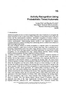
In this work we refrain from answering the question why Syntactic Pattern Recognition techniques fell out of favor with image processing community. We believe that in the domain of action recognition, where the character of the input is clearly sequential, the solution yielded by a sequential machines is called for and well justified. We motivate Syntactic Recognition approach by the apparent granularity of the processes, recognition of which we are attempting to address in our ongoing research. Indeed, in cognitive vision we can often easily determine the components of the complex behavior– based signal. The assumption is perhaps more valid in the context of conscious directed activity since the nature of the signal is such that it is generated by a taskdriven system, and the decomposition of the input to the vision system is as valid as the decomposition of the task, being performed by the observed source, into a set of simpler primitive subtasks (eg. [5, 14, 7]). Figure 1: Error correcting capabilities of syntactic constraints
AI view AI approaches to recognition were traditionally based on the idea of incorporating the knowledge from a variety of knowledge sources and bringing them together to bear on the problem at hand. For instance, the AI approach to segmentation and labeling of the speech signal is to augment the generally used acoustic knowledge with phonemic knowledge, lexical knowledge, syntactic knowledge, semantic knowledge and even pragmatic knowledge. Rabiner and Juang ([17]) show that in tasks of automatic speech recognition, the word correcting capability of higher-level knowledge sources is extremely powerful. In particular, they illustrate this statement by comparing performance of a recognizer both with and without syntactic constraints (figure1 1). As the deviation (noise) parameter SIGM A gets larger, the word error probability increases in both cases. In the case without syntactic constraints, the error probability quickly leads to 1, but with the syntactical constraints enforced, it increases gradually with an increase in noise. In this report we present a framework in which syntactic constraints can be enforced in tasks of machine vision. This framework makes it simple to utilize the heterogeneous set of the knowledge sources at appropriate levels of abstraction, while retaining the simplicity and elegance of probabilistic Finite State models, without the necessity to correspondingly limit the model’s complexity. 1
2
Related Work
Probabilistic aspects of syntactic pattern recognition for speech processing were presented in many publications, for instance in [13, 10]. The latter demonstrates some key approaches to parsing sentences of natural language and shows advantages of use of probabilistic CFGs. The text shows natural progression from HMM-based methods to probabilistic CFGs, demonstrating the techniques of computing the sequence probability characteristics, familiar from HMMs, such as forward and backward probabilities in the chart parsing framework. An efficient probabilistic version of Earley parsing algorithm was developed by Stolcke in his dissertation ([20]). The author develops techniques of embedding the probability computation and maximization into the Earley algorithm. He also describes grammar structure learning strategies and the rule probability learning technique, justifying usage of Stochastic Context-Free Grammars for natural language processing and learning. Aho and Peterson addressed the problem of illformedness of the input stream. In [1] they described a modified Earley’s parsing algorithm where substitution, insertion and deletion errors are corrected. The basic idea is to augment the original grammar by error productions for insertions, substitutions and deletions, such that any string over the terminal alphabet can be generated by the augmented grammar. Each such pro-
Reprinted from [17]
2
duction has some cost associated with it. The parsing proceeds in such a manner as to make the total cost minimal. It has been shown that the error correcting Earley parser has the same time and space complexity as the original version, namely O(N 3 ) and O(N 2 ) respectively, where N is the length of the string. Their approach is utilized in this thesis in the framework of uncertain input and multi-valued strings. The syntactic approach in Machine Vision has been studied for more than thirty years (Eg. [15, 3]), mostly in the context of pattern recognition in still images. The work by Bunke and Pasche ([6]) is built upon the previously mentioned development by Aho and Peterson ([1]), expanding it to multi-valued input. The resulting method is suitable for recognition of patterns in distorted input data and is shown in applications to waveform and image analysis. The work proceeds entirely in non-probabilistic context. More recent work by Sanfeliu et al ([19]) is centered around two-dimensional grammars and their applications to image analysis. The authors pursue the task of automatic traffic sign detection by a technique based on Pseudo Bidimensional Augmented Regular Expressions (PSB-ARE). AREs are regular expressions augmented with a set of constraints that involve the number of instances in a string of the operands to the star operator, alleviating the limitations of the traditional FSMs and CFGs which cannot count their arguments. More theoretical treatment of the approach is given in [18]. In the latter work, the authors introduce a method of parsing AREs which describe a subclass of a context-sensitive languages, including the ones defining planar shapes with symmetry. A very important theoretical work, signifying an emerging information theoretic trend in stochastic parsing, is demonstrated by Oomen and Kashyap in [16]. The authors present a foundational basis for optimal and information theoretic syntactic pattern recognition. They develop a rigorous model for channels which permit arbitrary distributed substitution, deletion and insertion syntactic errors. The scheme is shown to be functionally complete and stochastically consistent. There are many examples of attempts to enforce syntactic and semantic constraints in recognition of visual data. For instance, Courtney ([8]) uses a structural approach to interpreting action in a surveillance setting. Courtney defines high level discrete events, such as “object appeared”, “object disappeared” etc., which are extracted from the visual data. The sequences of the events are matched against a set of heuristically determined sequence templates to make
decisions about higher level events in the scene, such as “object A removed from the scene by object B”. The grammatical approach to visual activity recognition was used by Brand ([4]), who used a simple non-probabilistic grammar to recognize sequences of discrete events. In his case, the events are based on blob interactions, such as “objects overlap” etc.. The technique is used to annotate a manipulation video sequence, which has an a priori known structure. And finally, hybrid techniques of using combined probabilistic-syntactic approaches to problems of image understanding are shown in pioneering research by Fu (eg.[22, 12]).
3
Stochastic Context-Free Grammars
The probabilistic aspect is introduced into syntactic recognition tasks via Stochastic Context-Free Grammars. A Stochastic Context-Free Grammar (SCFG) is a probabilistic extension of a Context-Free Grammar. The extension is implemented by adding a probability measure to every production rule: A → λ [p] The rule probability p is usually written as P (A → λ). This probability is a conditional probability of the production being chosen, given that non-terminal A is up for expansion (in generative terms). Saying that stochastic grammar is context-free essentially means that the rules are conditionally independent and, therefore, the probability of the complete derivation of a string is just a product of the probabilities of rules participating in the derivation. Given a SCFG G, let us list some basic definitions: 1. The probability of partial derivation ν ⇒ µ ⇒ . . . λ is defined in inductive manner as (a) P (ν) = 1 (b) P (ν ⇒ µ ⇒ . . . λ) = P (A → ω)P (µ ⇒ . . . λ), where production A → ω is a production of G, µ is derived from ν by replacing one occurrence of A with ω, and ν, µ, . . . , λ ∈ VG∗ . 2. The string probability P (A ⇒∗ λ) (Probability of λ given A) is the sum of all left-most derivations A ⇒ . . . ⇒ λ. 3. The sentence probability P (S ⇒∗ λ) (Probability of λ given G) is the string probability given the axiom S of G. In other words, it is P (λ|G). 4. The prefix probability P (S ⇒∗L λ) is the sum of the strings having λ as a prefix,
3
P (S ⇒∗L λ) =
�
notation above, for each state Ski and production p of a grammar G = {T, N, S, P } of the form � i i : Xk → λ.Y µ Sk : (1) p : Y →ν
P (A ⇒∗ λω)
∗ ω∈VG
In particular, P (S ⇒∗L �) = 1.
4
where Y ∈ N , we predict a state Sii :
Earley-Stolcke Parsing Algorithm
Prediction step can take on a probabilistic form by keeping track of the probability of choosing a particular predicted state. Given the statistical independence of the nonterminals of the SCFG, we can write the probability of predicting a state Sii as conditioned on probability of Ski . This introduces a notion of forward probability, which has the interpretation similar to that of a forward probability in HMMs. In SFCG the forward probability αi is the probability of the parser accepting the string w1 ...w(i−1) and choosing state S at a step i. To continue the analogy with HMMs, inner probability, γi , is a probability of generating a substring of the input from a given nonterminal, using a particular production. Inner probability is thus conditional on the presence of a nonterminal X with expansion started at the position k, unlike the forward probability, which includes the generation history starting with the axiom. Formally, we can integrate computation of α and γ with non-probabilistic Earley predictor as follows:
The method most generally and conveniently used in stochastic parsing is based on an Earley parser ([11]), extended in such a way as to accept probabilities. In parsing stochastic sentences we adopt a slightly modified notation of [20]. The notion of a state is an important part of the Earley parsing algorithm. A state is denoted as: i : Xk → λ.Y µ where ’.’ is the marker of the current position in the input stream, i is the index of the marker, and k is the starting index of the substring denoted by nonterminal X. Nonterminal X is said to dominate substring wk ...wi ...wl , where, in the case of the above state, wl is the last terminal of substring µ. In cases where the position of the dot and structure of the state is not important, for compactness we will denote a state as: Ski ≡ i : Xk → λ.Y µ
�
Parsing proceeds as an iterative process sequentially switching between three steps - prediction, scanning and completion. For each position of the input stream, an Earley parser keeps a set of states, which denote all pending derivations. States produced by each of the parsing steps are called, respectively, predicted, scanned and completed. A state is called complete (not to be confused with completed), if the dot is located in the rightmost position of the state. A complete state is the one that “passed” the grammaticality check and can now be used as a “ground truth” for further abstraction. A state “explains” a string that it dominates as a possible interpretation of symbols wk ...wi , “suggesting” a possible continuation of the string if the state is not complete.
4.1
i : Yi → .ν
i : Xk → λ.Y µ [α, γ] Y →ν
=⇒
i : Y → .ν
[α� , γ � ]
where α� is computed as a sum of probabilities of all the paths, leading to the state i : Xk → λ.Y µ multiplied by the probability of choosing the production Y → ν, and γ � is the rule probability, seeding the future substring probability computations: � α� = ∀λ,µ α(i : Xk → λ.Y µ)P (Y → ν) γ � = P (Y → ν) 4.1.1 Recursive correction Because of possible left recursion in the grammar the total probability of a predicted state can increase with it being added to a set infinitely many times. Indeed, if a non-terminal A is considered for expansion and given productions for A
Prediction
A
In the Earley parsing algorithm the prediction step is used to hypothesize the possible continuation of the input based on current position in the parse tree. Prediction essentially expands one branch of the parsing tree down to the set of its leftmost leaf nodes to predict the next possible input terminal. Using the state
→ →
Aa a
we will predict A → .a and A → .Aa at the first prediction step. This will cause the predictor to consider these newly added states for possible descent,
4
p2 A
G2 : S → → → A → → B → → C → → →
C p1 p4
p3
B
G1 : A → → B → → C →
BB CB AB C a
[p1 ] [p2 ] [p3 ] [p4 ] [p5 ]
0 p3 0
p1 0 0
AB C d AB a bB b BC B c
[p1 ] [p2 ] [p3 ] [p4 ] [p5 ] [p6 ] [p7 ] [p8 ] [p9 ] [p10 ]
PL S A B C
S
RL S A B C
S 1
A p1 p4
B
C p2
p8 + p9 A −p1 −1+p4 −1 −1+p4
B p2 p8 + p2 p9
C p2
1 p8 + p9
1
Table 1: Left Corner Relation (PL ) and its Reflexive Transitive Closure (RL ) matrices for a simple SCFG.
p2 p4 0
that the probability of emitting terminal a, such that � X →Yν Y → aη
Figure 2: Left Corner Relation graph of the grammar G1 . Matrix PL is shown on the right of the productions of the grammar.
(from which follows that X → aην) is a sum of probabilities along all the paths connecting X with Y , multiplied by probability of direct emittance of a from Y , P (Y → aη). Formally, � ∗ P (a) = P (Y → aη) ∀X P (X ⇒ Y ) ∗ = P (Y → aη) (P0 (X ⇒ Y )+ P1 (X ⇒∗ Y )+ P2 (X ⇒∗ Y ) + . . .
which will produce the same two states again. In nonprobabilistic Earley parser it normally means that no further expansion of the production should be made and no duplicate states should be added. In probabilistic version, however, although adding a state will not add any more information to the parse, its probability has to be factored in by adding it to the probability of the previously predicted state. In the above case that would mean an infinite sum due to left-recursive expansion.
where Pk (X ⇒ Y ) is probability of a path from X to Y of length k = 1, . . . , ∞ In matrix form all the k−step path probabilities on a graph can be computed from its adjacency matrix as PLk . Using the matrix PLk , the reflexive transitive closure of the LC relation can be easily found as a matrix of infinite sums, RL , which has a closed form solution:
In order to demonstrate the solution we first need to introduce the concept of Left Corner Relation. Two nonterminals are said to be in a Left Corner Relation X →L Y iff there exists a production for X of the form X → Y λ.
RL = PL0 + PL1 + PL2 + . . . =
∞ �
PLk = (I − PL )−1
k=0
We can compute a total recursive contribution of each left-recursive production rule where nonterminals X and Y are in Left Corner Relation. The necessary correction for non-terminals can be computed in a matrix form. The form of recursive correction matrix RL can be derived using simple example presented in Figure 2. The graph of the relation presents direct left corner relations between nonterminals of G1 . The LC Relation matrix PL of the grammar G1 is essentially the adjacency matrix of this graph. If there exists an edge between two nonterminals X and Y it follows
Thus, the correction to the completion step should be applied by descending the chain of left corner productions, indicated by a non-zero value in RU : i : Xk → λ.Zµ [α, γ] ∀Z s.t. RL (Z, Y ) = 0 Y →ν
=⇒
i : Y → .ν
[α� , γ � ]
where forward and inner probabilities for the left recursive productions are corrected by an appropriate entry of the matrix RL :
5
�
α γ�
= =
G2 : S → → → A → → B → → C → → →
�
∀λ,µ α(i : Xk → λ.Zµ)RL (Z, Y )P (Y → ν) P (Y → ν)
Matrix RL can be computed once for the grammar and used at each iteration of the prediction step.
4.2
Scanning
Scanning step simply reads the input symbol and matches it against all pending states for the next iteration. For each state Xk → λ.aµ and the input symbol a we generate a state i + 1 : Xk → λa.µ: i : Xk → λ.aµ =⇒ i + 1 : Xk → λa.µ
[p1 ] [p2 ] [p3 ] [p4 ] [p5 ] [p6 ] [p7 ] [p8 ] [p9 ] [p10 ]
S
RU S A B C
S 1
A
B
C p2
p9 A
B p2 p9
C p2
1 p9
1
1
Table 2: Unit Production (PU ) and its Reflexive Transitive Closure (RU ) matrices for a simple SCFG.
It is readily converted to the probabilistic form. The forward and inner probabilities remain unchanged from the state being confirmed by the input, since no selections are made at this step. The probability, however, may change if there is a likelihood associated with the input terminal. This will be exploited in the next chapter dealing with uncertain input. In probabilistic form the scanning step is formalized as:
�
j : Xk → λ.Y µ [α, γ] =⇒ i : Xk → λY.µ i : Yj → ν. [α�� , γ �� ]
α� γ�
= =
[α� , γ � ]
� α(i : Xk → λ.Y µ)γ �� (i : Yj → ν.) �∀λ,µ �� ∀λ,µ γ(i : Xk → λ.Y µ)γ (i : Yj → ν.)
4.3.1 Recursive correction Here, as in prediction, we might have a potential danger of entering an infinite loop. Indeed, given the productions
i : Xk → λ.aµ [α, γ] =⇒ i + 1 : Xk → λa.µ [α, γ] where α and γ are forward and inner probabilities. Note the increase in i index. This signifies the fact that scanning step inserts the states into the new state set for the next iteration of the algorithm.
4.3
AB C d AB a bB b BC B c
PU S A B C
A B
Completion
→ → →
B a A
and the state i : Aj → a., we complete the state set j, containing:
Completion step, given a set of states which just have been confirmed by scanning, updates the positions in all the pending derivations all the way up the derivation tree. The position in expansion of a pending state j : Xk → λ.Y µ is advanced if there is a state, starting at position j, i : Yj → ν., which consumed all the input symbols related to it. Such a state can now be used to confirm other states, expecting Y as their next nonterminal. Since the index range is attached to Y , we can effectively limit the search for the pending derivations to the state set, indexed by the starting index of the completing state, j: � j : Xk → λ.Y µ =⇒ i : Xk → λY.µ i : Yj → ν.
j : Aj j : Aj j : Bj
→ → →
. B . a . A
Among others this operation will produce another state i : Aj → a. , which will cause the parse to go into infinite loop. In non-probabilistic Earley parser that would mean that we just simply do not add the newly generated states and proceed with the rest of them. However, this will introduce the truncation of the probabilities as in the case with prediction. It has been shown that this infinite loop appears due to socalled unit productions ([21]). Two nonterminals are said to be in a Unit Production Relation X →U Y iff there exists a production for X of the form X → Y . As in the case with prediction we compute the closed-form solution for a Unit Production recursive correction matrix RU (figure 2), considering the Unit Production relation, expressed by a matrix PU . RU is
Again, propagation of forward and inner probabilities is simple. New values of α and γ are computed by multiplying the corresponding probabilities of the state being completed by the total probability of all paths, ending at i : Yj → ν. . In its probabilistic form, completion step generates the following states:
6
found as RU = (I − PU )−1 . The resulting expanded completion algorithm accommodates for the recursive loops:
recognition. Most often these components are detected “after the fact”, that is, recognition of the activity only succeeds when the whole corresponding sub-sequence is present in the causal signal. At the point when the activity is detected by the low level recognizer, the like j : Xk → λ.Zµ [α, γ] lihood of the activity model represents the probability ∀Z s.t. RU (Z, Y ) = 0 =⇒ i : Xk → λZ.µ [α� , γ � ] that this part of the signal has been generated by the i : Yj → ν. [α�� , γ �� ] corresponding model. In other words, with each activity likelihood, we will also have the sample range of the input signal, or a corresponding time interval, to which where computation of α� and γ � is corrected by a corit applies. This fact will be the basis of the technique responding entry of RU : for enforcing temporal consistency of the input, devel� oped later in this chapter. We will refer to the model α� = α(i : Xk → λ.Zµ)RU (Z, Y )γ �� (i : Yj → ν.) �∀λ,µ activity likelihood as a terminal, and to the length of = γ(i : Xk → λ.Y µ)RU (Z, Y )γ �� (i : Yj → ν.) γ� ∀λ,µ corresponding sub-sequence as a terminal length.
As RL , unit production recursive correction matrix RU can be computed once for each grammar.
5
5.2
The previous section described the parsing algorithm, where no uncertainty about the input symbols is taken into consideration. New symbols are read off by the parser during the scanning step, which changes neither forward nor inner probabilities of the pending states. If the likelihood of the input symbol is also available, as in our case, it can easily be incorporated into the parse during scanning by multiplying the inner and forward probability of the state being confirmed by the input likelihood. We reformulate the scanning step as follows: having read a symbol a and its likelihood P (a) off the input stream, we produce the state
Temporal Parsing of Uncertain Input
The approach described in the previous chapter can be effectively used to find the most likely syntactic groupings of the elements in a non-probabilistic input stream. The probabilistic character of the grammar comes into play when disambiguation of the string is required by the means of the probabilities attached to each rule. These probabilities reflect the “typicality” of the input string. By tracing the derivations, to each string we can assign a value, reflecting how typical the string is according to the current model. In this chapter we to address two main problems in application of the parsing algorithm described so far to action recognition:
i : Xk → λ.aµ [α, γ] =⇒ i + 1 : Xk → λa.µ [α� , γ � ] and compute new values of α� and γ � as: α� γ�
• Uncertainty in the input string. The input symbols which are formed by low level temporal feature detectors are uncertain. This implies that some modifications to the algorithm which account for this are necessary.
= =
α(i : Xk → λ.aµ)P (a) γ(i : Xk → λ.aµ)P (a)
The new values of forward and inner probabilities will weigh competing derivations not only by their typicality, but also by our certainty about the input at each sample.
• Temporal consistency of the event stream. Each symbol of the input stream corresponds to some time interval. Since here we are dealing with a single stream input, only one input symbol can be present in the stream at a time and no overlapping is allowed, which the algorithm must enforce.
5.1
Uncertainty in the Input String
5.3
Substitution
Introducing likelihoods of the terminals at the scanning step makes it simple to employ the multi-valued string parsing ([6]) where each element of the input is in fact a multi-valued vector of vocabulary model likelihoods at each time step of an event stream. Using these likelihoods, we can condition the maximization of the parse not only on frequency of occurrence of some sequence in the training corpus, but also on measurement or estimation of the likelihood of each of the sequence component in the test data.
Terminal Recognition
Before we proceed to develop the temporal parsing algorithm, we need to say a few words about the formation of the input. In this thesis we are attempting to combine the detection of independent component activities in a framework of syntax-driven structure
7
The multi-valued string approach allows for dealing with so-called substitution errors which manifest themselves in replacement of a terminal in the input string with an incorrect one. It is especially relevant to the problems addressed by this thesis where sometimes the correct symbol is rejected due to a lower likelihood than that of some other one. In the proposed approach, we allow the input at discrete instance of time to include all non-zero likelihoods and to let the parser select the most likely one, based not only on the corresponding value, but also on the probability of the whole sequence, as additional reinforcement to the local model estimate. From this point and on, the input stream will be viewed as a multi-valued string (a lattice) which has a vector of likelihoods, associated with each time step (e.g. figure 3). The length of the vector is in general equal to the number of vocabulary models. The model likelihoods are incorporated with the parsing process at the scanning step, as was shown above, by considering all non-zero likelihoods for the same state set, that is: �
i : Xk → λ.aµ [α, γ] ∀a, s.t. P (a) > 0
=⇒ i + 1 : Xk → λa.µ
Figure 3: Example of the lattice parse input for three model vocabulary. Consider a grammar A → abc | acb. The dashed line shows a parse acb. The two rectangles drawn around samples 2 and 4 show the “spurious symbols” for this parse which need to be ignored for the derivation to be contiguous. We can see that if the spurious symbols are simply removed from the stream, an alternative derivation for the sequence - abc, shown by a dotted line, will be interrupted. (Note the sample 3 which contains two concurrent symbols which are handled by the lattice parsing.)
[α� , γ � ]
The parsing is performed in a parallel manner for all suggested terminals.
5.4
mation about the overall validity of this string, that is, we cannot simply discard samples 2 and 4 from the stream, because combined with sample 1, they form an alternative string, abc. For this alternative derivation, sample 3 would present a problem if not dealt with. There are at least three possible solutions to the insertion problem in our context.
Insertion
It has been shown that “while significant progress has been made in the processing of correct text, a practical system must be able to handle many forms of ill-formedness gracefully” [2]. In our case, the need for this robustness is paramount. Indeed, the parsing needs to be performed on a lattice, where the symbols which we need to consider for inclusion in the string come at random times. This results in appearance of “spurious” (i.e. ungrammatical) symbols in the input stream, a problem commonly referred to as insertion. We need to be able to consider these inputs separately, at different time steps, and disregard them if their appearance in the input stream for some derivation is found to be ungrammatical. At the same time, we need to preserve the symbol in the stream for considering it in other possible derivations, perhaps even of a completely different string. The problem is illustrated by figure 3. In this figure we observe two independent derivations on an uncertain input stream. While deriving the string acb, connecting samples 1, 3 and 5, we need to disregard samples 2 and 4, which would interfere with the derivation. However we do not have an a priori infor-
• Firstly, we can employ some ad hoc method which “synchronizes” the input, presenting the terminals coming with a slight spread around a synchronizing signal, as one vector. That would significantly increase the danger of not finding a parse if the spread is significant. • Secondly, we may attempt gathering all the partially valid strings, performing all the derivations we can on the input and post-processing the resulting set to extract the most consistent maximum probability set of partial derivations. Partial derivations acquired by this technique will show a distinct split at the position in the input where the supposed ungrammaticality occurred. Being robust for finding ungrammatical symbols in a single stream, in our experiments, this method did not produce the desired results. The lattice extension, extremely noisy input and a relatively shal-
8
1
low grammar made it less useful, producing large number of string derivations, which contained a large number of splits and were difficult to analyze.
0.8 0.6 0.4 0.2
• And, finally, we can attempt to modify the original grammar to explicitly include the ERROR symbol (e.g. [1]).
0 0
4
6
8
10 t
12
14
16
18
20
2
4
6
8
10 t
12
14
16
18
20
1
In our algorithm the last approach proved to be the most suitable as it allowed us to incorporate some additional constraints on the input stream easily, as will be shown in the next section. We formulate simple rules of the grammar modifications and perform the parsing of the input stream using this modified grammar. ˆ is formed Given the grammar G, robust grammar G by following rules:
0.8 0.6 0.4 0.2 0 0
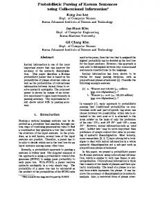
Figure 4: Example of temporally inconsistent terminals. Given a production A → ab | abA unconstrained parse will attempt to consume maximum amount of samples by non-SKIP productions. The resulting parse, ababab, is shown by the dashed line. The solid line shows the correct parse, abab, which includes only non-overlapping terminals (horizontal lines show the sample range of each candidate terminal).
1. Each terminal in productions of G is replaced by ˆ a pre-terminal in G: ˆ: G: ⇒ G ˆ A → bC A → BC ˆ a skip rule is formed: 2. For each pre-terminal of G ˆ G: ˆ → b | SKIP b | b SKIP B This is essentially equivalent to adding a producˆ tion B → SKIP b SKIP if SKIP is allowed to expand to �.
serves as a function that “penalizes” the parser for each symbol considered ungrammatical. This might result in the phenomenon where some of the “noise” gets forced to take part in a derivation as a grammatical occurrence. The effect of this can be relieved if we take into account the temporal consistency of the input stream, that is, only one event happens at a given time. Since each event has a corresponding length, we can further constrain the occurrence of the terminals in the input so that no “overlapping” events take place. The problem is illustrated in figure 4. In Earley framework, we can modify the parsing algorithm to work in incremental fashion as a filter to the completion step, while keeping track of the terminal lengths during scanning and prediction. In order to accomplish the task we need to introduce two more state variables - h for “high mark” and l for “low mark”. Each of the parsing steps has to be modified as follows:
ˆ which includes all repe3. Skip rule is added to G, titions of all terminals: ˆ: G SKIP → b | c | ... | b SKIP | c SKIP ... Again, if SKIP is allowed to expand to �, the last two steps are equivalent to adding: ˆ: G ˆ B → SKIP b SKIP SKIP → � | b SKIP . . .
6.1
This process can be performed automatically as a pre-processing step, when the grammar is read in by the parser, so that no modifications to the grammar are explicitly written.
6
2
Scanning
Scanning step is modified to include reading the time interval associated with the incoming terminal. The updates of l and h are propagated during the scanning as follows:
Enforcing Temporal Consistency
i : Xk → λ.aµ
Parsing the lattice with the robust version of the original grammar results in the parser consuming a maximum amount of the input. Indeed, the SKIP production, which is usually assigned a low probability,
[l, h]
=⇒
i + 1 : Xk → λa.µ
[l, ha ]
where ha is a high mark of the terminal. In addition to this, we set the time-stamp of the whole new (i +
9
6.5
1)-th state set to ha : St = ha , to be used later by prediction step.
6.2
Viterbi parse is applied to the state sets in a chart parse in a manner similar to HMMs. Viterbi probabilities are propagated in the same way as inner probabilities, with the exception that instead of summing the probabilities during completion step, maximization is performed. That is, given a complete state Sji , we can formalize the process of computing Viterbi probabilities vi as follows:
Completion
Similarly to scanning, completion step advances the high mark of the completed state to that of the completing state, thereby extending the range of the completed non-terminal. �
j : Xk → λ.Y µ [l1, h1] i : Yj → ν. [l2, h2]
=⇒
i : Xk → λY.µ
[l1 , h2 ]
vi (Ski ) = maxSji (vi (Sji )vj (Skj ))
This completion is performed for all states i : Yj → ν. subject to constraints l2 ≥ h1 and Y, X = SKIP .
6.3
and the Viterbi path would include the state Ski = argmaxSji (vi (Sji )vj (Skj ))
Prediction
Prediction step is responsible for updating the low mark of the state to reflect the timing of the input stream. � i : Xk → λ.Y µ =⇒ i : Y → .ν [St , St ] Y →ν
The state Ski keeps a back-pointer to the state Sji , which completes it with maximum probability, providing the path for backtracking after the parse is complete. The computation proceeds iteratively, within the normal parsing process. After the final state is reached, it will contain pointers to its immediate children, which can be traced to reproduce the maximum probability derivation tree.
Here, St is the time-stamp of the state set, updated by the scanning step.
6.4
Misalignment Cost
6.5.1
Viterbi Parse in Presence of Unit Productions The otherwise straight forward algorithm of updating Viterbi probabilities and the Viterbi path is complicated in the completion step by the presence of the Unit productions in the derivation chain. Computation of the forward and inner probabilities has to be performed in closed form, as described previously, which causes the unit productions to be eliminated from the Viterbi path computations. This results in producing an inconsistent parse tree with omitted unit productions, since in computing the closed form correction matrix, we collapse such unit production chains. In order to remedy this problem, we need to consider two competing requirements to the Viterbi path generation procedure.
The essence of the filtering technique described in the previous section is that only the paths that are consistent in the timing of their terminal symbols are considered. This does not interrupt the parses of the sequence since filtering, combined with robust grammar, leaves the subsequences which form the parse connected via the skip states. In the process of temporal filtering, it is important to remember that the terminal lengths are themselves uncertain. A useful extension to the temporal filtering is to implement a softer penalty function, rather than a hard cut-off of all the overlapping terminals, as described above. It is easily achieved at the completion step where the filtering is replaced by a weighting function f (θ), of a parameter θ = h1 − l2 , which is multiplied into forward and inner probabilities. For 2 instance, f (θ) = e−ψθ , where ψ is a penalizing parameter, can be used to weigh “overlap” and “spread” equally. The resulting penalty is incorporated with computation of α and γ: α�
=
f (θ)
γ�
=
f (θ)
� �� �∀λ,µ α(i : Xk → λ.Zµ)RU (Z, Y )γ �� (i : Yj ∀λ,µ
Viterbi Parsing
1. On one hand, we need a batch version of the probability calculation performed, as previously described, to compute transitive recursive closures on all the probabilities, by using recursive correction matrices. In this case, Unit productions do not need to be considered by the algorithm, since their contributions to the probabilities are encapsulated in the recursive correction matrix RU .
→ ν.)
γ(i : Xk → λ.Y µ)RU (Z, Y )γ (i : Yj → ν.)
2. On the other hand, we need a finite number of states to be considered as completing states in a
More sophisticated forms of f (θ) can be formulated to achieve arbitrary spread balancing as needed.
10
which can make the parser go into an infinite loop. Such loops should be avoided while formulating the grammar. A better solution is being sought.
function StateSet.Complete() ... if(State.IsUnit()) State.Forward = 0; State.Inner = 0; else State.Forward = ComputeForward(); State.Inner = ComputeInner(); end
7
On-line Processing
7.1
NewState = FindStateToComplete(); NewState.AddChild(State); StateSet.AddState(NewState); ... end
Pruning
As we gain descriptive advantages with using SCFGs for recognition, the computational complexity, as compared to Finite State Models, increases. The complexity of the algorithm grows linearly with increasing length of the input string. This presents us with the necessity in certain cases of pruning low probability derivation paths. In Earley framework such a pruning is easy to implement. We simply rank the states in the state set according to their per sample forward probabilities and remove those that fall under a certain threshold. However, performing pruning one should keep in mind that the probabilities of the remaining states will be underestimated.
function StateSet.AddState(NewState) ... if(StateSet.AlreadyExists(NewState) OldState = StateSet.GetExistingState(NewState); CompletingState = NewState.GetChild(); if(OldState.HasSameChildren(CompletingState)) OldState.ReplaceChildren(CompletingState); end OldState.AddProbabilities(NewState.Forward, NewState.Inner); else StateSet.Add(NewState); end ... end
Figure 5: Simplified pseudo-code of the modifications to the completion algorithm.
7.2
natural order so that we can preserve the path through the parse to have a continuous chain of parents for each participating production. In other words, the unit productions, which get eliminated from the Viterbi path during the parse while computing Viterbi probability, need to be included in the complete derivation tree.
Limiting the Range of Syntactic Grouping
Context-free grammars have a drawback of not being able to express countable relationships in the string by a hard bound by any means other than explicit enumeration. One implication of this drawback is that we cannot formally limit the range of the application of a SKIP productions and formally specify how many SKIP productions can be included in a derivation for the string to still be considered grammatical. When parsing with robust grammar is performed, some of the non-terminals being considered for expansion cover large portions of the input string consuming only a few samples by non-SKIP rules. The states, corresponding to such non-terminals, have low probability and typically have no effect on the derivation, but are still considered in further derivations, increasing the computational load. This problem is especially relevant when we have a long sequence and the task is to find a smaller subsequence inside it which is modeled by an SCFG. Parsing the whole sequence might be computationally expensive if the sequence is of considerable length. We can attempt to remedy this problem by limiting the range of productions. In our approach, when faced with the necessity to perform such a parse, we use implicit pruning by operating a parser on a relatively small sliding window. The parse performed in this manner has two important features:
We solve both problems by computing the forward, inner and Viterbi probabilities in closed form by applying the recursive correction RU to each completion for non-unit completing states and then, considering only completing unit production states for inserting them into the production chain. Unit production states will not update their parent’s probabilities, since those are already correctly computed via RU . Now the maximization step in computing the parent’s Viterbi probability needs to be modified to keep a consistent tree. To accomplish this, when using the unit production to complete a state, the algorithm inserts the Unit production state into a child slot of the completed state only if it has the same children as the state it is completing. The overlapping set of children is removed from the parent state. It extends the derivation path by the Unit production state, maintaining consistent derivation tree. Pseudo-code of the modifications to the completion algorithm which maintains the consistent Viterbi derivation tree in presence of Unit production states is shown in Figure 5. However, the problem stated in subsection 4.3.1 still remains. Since we cannot compute the Viterbi paths in closed form, we have to compute them iteratively,
• The “correct” string, if exists, ends at the current sample.
11
• The beginning sample of such a string is unknown, but is within the window.
cannot be converted to a sequence of transitions of an HMM. Presence of this mechanism makes richer structural derivations, such as counting and recursion, possible and simple to formalize. Another, more subtle difference has its roots in the way HMMs and SCFGs assign probabilities. SCFGs assign probabilities to the production rules, so that for each non-terminal, the probabilities sum up to 1. It translates into probability being distributed over sentences of the language - probabilities of all the sentences (or structural entities) of the language sum up to 1. HMMs in this respect are quite different - the probability gets distributed over all the sequences of a length n ([10]). In the HMM framework, the tractability of the parsing is afforded by the fact that the number of states remains constant throughout the derivation. In the Earley SCFG framework, the number of possible Earley states increases linearly with the length of the input string, due to the starting index of each state. This makes it necessary in some instances to employ pruning techniques which allow us to deal with increasing computational complexity when parsing long input strings.
From these observations, we can formalize the necessary modifications to the parsing technique to implement such a sliding window parser: 1. Robust grammar should only include the SKIP productions of the form A → a | SKIP a since the end of the string is at the current sample, which means that there will not be trailing noise, which is normally accounted for by a production A → a SKIP . 2. Each state set in the window should be seeded with a starting symbol. This will account for the unknown beginning of the string. After performing a parse for the current time step, Viterbi maximization will pick out the maximum probability path, which can be followed back to the starting sample exactly. This technique is equivalent to a run-time version of Viterbi parsing used in HMMs ([9]). The exception is that no “backwards” training is necessary since we have an opportunity to “seed” the state set with an axiom at an arbitrary position.
8
References
Conclusions
The use of formal languages and syntax-based action recognition is reasonable if decomposition of the action under consideration into a set of primitives that lend themselves to automatic recognition is possible. In contrast, applying the described techniques to the problems where no apriory knowledge about the process structure can be obtained will most likely fail. Existence of such a structure in the process is a prerequisite for using Syntactic Pattern recognition in general.
8.1
[1]
A. V. Aho and T. G. Peterson. A minimum distance error-correcting parser for context-free languages. SIAM Journal of Computing, 1, 1972.
[2]
J. Allen. Special issue on ill-formed input. American Journal of Computational Linguistics, 9(3–4):123– 196, 1983.
[3]
M. L. Baird and M. D. Kelly. A paradigm for semantic picture recognition. PR, 6(1):61–74, 1974.
[4]
M. Brand. Understanding manipulation in video. In AFGR96, pages 94–99. 1996.
[5]
R. A. Brooks. A robust layered control system for a mobile robot. IEEE Journal of Robotics and Automation, 1989.
[6]
H. Bunke and D. Pasche. Parsing multivalued strings and its application to image and waveform recognition. Structural Pattern Analisys, 1990.
[7]
J. H. Connell. A Colony Architecture for an Artificial Creature. Ph.d., MIT, 1989.
[8]
J. D. Courtney. Automatic video indexing via object motion analysis. PR, 30(4):607–625, 1997.
[9]
T. J. Darrell and A. P. Pentland. Space-time gestures. Proc. Comp. Vis. and Pattern Rec., pages 335–340, 1993.
Relation to HMM
While SCFGs look very different from HMMs, they have some remarkable similarities. In order to consider the similarities in more detail, let us look at a subset of SCFGs - Stochastic Regular Grammars. SRG is a 4tuple G = N, T, P, S, where the set of productions P is of the form A → aB, or A → a. If we consider the fact that HMM is a version of probabilistic Finite State Machine, we can apply simple non-probabilistic rules to convert an HMM into an SRG. More precisely, taking transition A →a B, with probability pm of an HMM, we can form an equivalent production A → aB [pm ]. Conversion of an SCFG in its general form is not always possible. An SCFG rule A → aAa, for instance
[10] Charniak. E. Statistical Language Learning. MIT Press, Cambridge, Massachusetts and London, England, 1993.
12
[11] Jay Clark Earley. An Efficient Context-Free Parsing Algorithm. Ph.d., Carnegie-Mellon University, 1968. [12] K. S. Fu. A step towards unification of syntactic and statistical pattern recognition. IEEE Transactions on Pattern Analysis and Machine Intelligence, PAMI-8(3):398–404, 1986. [13] F. Jelinek, J. D. Lafferty, and R. L. Mercer. Basic methods of probabilistic context free grammars. In Pietro Laface Mori and Renato Di, editors, Speech Recognition and Understanding. Recent Advances, Trends, and Applications, volume F75 of NATO Advanced Study Institute, pages 345–360. Springer Verlag, Berlin, 1992. [14] P. Maes. The dynamic of action selection. AAAI Spring Symposium on AI Limited Rationality, 1989. [15] R. Narasimhan. Labeling schemata and syntactic descriptions of pictures. InfoControl, 7(2):151–179, 1964. [16] B. J. Oomen and R. L. Kashyap. Optimal and information theoretic syntactic pattern recognition for traditional errors. SSPR 6th International Workshop on Advances in Structural and Syntactic Pattern Recognition., 1996. [17] L. R. Rabiner and B. H. Juang. Fundamentals of speech recognition. Prentice Hall, Englewood Cliffs, 1993. [18] A. Sanfeliu and R. Alquezar. Efficient recognition if a class of context-sensitive languages described by augmented regular expressions. SSPR 6th International Workshop on Advances in Structural and Syntactic Pattern Recognition., 1996. [19] A. Sanfeliu and M. Sainz. Automatic recognition of bidimensional models learned by grammatical inferrence in outdor scenes. SSPR 6th International Workshop on Advances in Structural and Syntactic Pattern Recognition., 1996. [20] A. Stolcke. Bayesian Learning of Probabilistic Language Models. Ph.d., University of California at Berkeley, 1994. [21] A. Stolcke. An efficient probabilistic context-free parsing algorithm that computes prefix probabilities. Computational Linguistics, 21(2), 1995. [22] W. G. Tsai and K. S. Fu. Attributed grammars - a tool for combining syntatctic and statistical approaches to pattern recognition. In IEEE Transactions on Systems, Man and Cybernetics, volume SMC-10, number 12, pages 873–885. 1980.
13