FUNCTIONAL magnetic resonance imaging (fMRI) is an exciting relatively new medical imaging technique that is providing much new information about the ...
IEEE TRANSACTIONS ON MEDICAL IMAGING, VOL. 18, NO. 2, FEBRUARY 1999
101
Activation Detection in Functional MRI Using Subspace Modeling and Maximum Likelihood Estimation Babak A. Ardekani, Member, IEEE,* Jeff Kershaw, Kenichi Kashikura, and Iwao Kanno
Abstract— A statistical method for detecting activated pixels in functional MRI (fMRI) data is presented. In this method, the fMRI time series measured at each pixel is modeled as the sum of a response signal which arises due to the experimentally controlled activation-baseline pattern, a nuisance component representing effects of no interest, and Gaussian white noise. For periodic activation-baseline patterns, the response signal is modeled by a truncated Fourier series with a known fundamental frequency but unknown Fourier coefficients. The nuisance subspace is assumed to be unknown. A maximum likelihood estimate is derived for the component of the nuisance subspace which is orthogonal to the response signal subspace. An estimate for the order of the nuisance subspace is obtained from an information theoretic criterion. A statistical test is derived and shown to be the uniformly most powerful (UMP) test invariant to a group of transformations which are natural to the hypothesis testing problem. The maximal invariant statistic used in this test has an F distribution. The theoretical F distribution under the null hypothesis strongly concurred with the experimental frequency distribution obtained by performing null experiments in which the subjects did not perform any activation task. Application of the theory to motor activation and visual stimulation fMRI studies is presented. Index Terms— Brain, functional MRI, maximum likelihood estimation, statistical analysis.
I. INTRODUCTION
F
UNCTIONAL magnetic resonance imaging (fMRI) is an exciting relatively new medical imaging technique that is providing much new information about the function of the human brain. The technique hinges upon the sensitivity of the magnetization decay rates to changes in physiological conditions. For example, the effective decay rate of the longitudinal magnetization is sensitive to increases in the inflow of blood during activation or sensory stimulation. The resulting signal Manuscript received March 2, 1998; revised October 30, 1998. This work was supported in part by the Human Brain Project, United States National Institutes of Health under Grant P20-MH57180. The work of B. A. Ardekani was supported by the Japanese Science and Technology Agency under an STA Research Fellowship. The Associate Editor responsible for coordinating the review of this paper and recommending its publication was X. Hu. Asterisk indicates corresponding author. *B. A. Ardekani was with the Department of Radiology and Nuclear Medicine, Research Institute for Brain and Blood Vessels, 6-10 Senshukubota machi, Akita 010, Japan . He is now with the Center for Advanced Brain Imaging, The Nathan S. Kline Institute, 140 Old Orangeburg Road, Orangeburg, NY 10962 USA. J. Kershaw, K. Kashikura, and I. Kanno are with the Department of Radiology and Nuclear Medicine, Research Institute for Brain and Blood Vessels, Akita 010, Japan. Publisher Item Identifier S 0278-0062(99)03798-2.
Fig. 1. General periodic activation-baseline pattern for an fMRI experiment.
change has been utilized in methods such as EPISTAR [1] and FAIR [2] in order to quantify cerebral blood flow (CBF) , which has a rates. Another example is the decay rate, blood oxygenation level dependence (BOLD) [3]. Apparently the increase in blood flow in activated areas of the brain exceeds the corresponding increase in oxygen consumption. Thus, venous blood has an elevated oxygen content which and a corresponding increase in results in an increased -weighted MRI. By rapidly acquiring a the intensity of series of MR images with pulse sequences that are sensitive , transient hemodynamic changes can to small changes in be observed. Since the signal change is localized to areas of the brain involved in the neuronal activity, it is possible to associate specific parts of the brain with specific functions. In effect, it is possible to build a map of human brain function. In the majority of reported functional human brain mapping studies using fMRI, blocks of baseline and activation images are are scanned periodically. Typically, a number of frames acquired while the subject is at rest or under some baseline condition. This is followed by a number of activation frames during which the subject is receiving a sensory stimulus or performing a specified motor or cognitive task. This pattern is then repeated for a number of cycles. During each cycle, the . In some total number of frames is, therefore, activation cases, the frame order is reversed, that is, the baseline frames in each cycle. The frames precede the activation-baseline pattern can be represented by a periodic rectangular waveform of period with values of one and zero representing activation and baseline conditions, respectively (Fig. 1). Once a frame sequence is acquired, it is necessary to analyze the data in order to detect the picture elements (pixels) with
0278–0062/99$10.00 1999 IEEE
102
IEEE TRANSACTIONS ON MEDICAL IMAGING, VOL. 18, NO. 2, FEBRUARY 1999
Fig. 2. Schematic of how we imagine the response is generated from the input activation-baseline pattern.
significant responses to the activation-baseline pattern. If we assume that images are acquired during an fMRI experiment, then the data at each pixel can be represented by a discreteof length . Each measured sequence time sequence can be thought of as containing three components: 1) a hemodynamic response signal component which arises due to the experimentally controlled activation-baseline pattern; 2) a nuisance component representing effects of no interest such as the average signal intensity, physiological biorhythms, and systematic drifts in the signal level; and 3) noise. One can think of the signal component as the response of a system whose input is the activation-baseline pattern (Fig. 2). A widely used method for detecting activated pixels in fMRI is the cross-correlation method [4]. In this method, one computes the cross-correlation between the measured time series (after estimation and removal of a nuisance component) and a reference signal which represents an estimate of the response signal component in . Those pixels that show high correlations are declared to be activated. The main drawback of this method is that the cross-correlation coefficients depend on the response signal (the output of the system in Fig. 2) which is unknown. Bandettini et al. [4] suggested the use of one of several possible estimates for the reference signal. The first and most easily implemented method is to use a delayed version of the activation-baseline pattern, that is, to model the system in Fig. 2 as a simple delay. The disadvantage of this method is that the delay, which may vary from pixel to pixel, must be known a priori. The second suggestion is to select the reference signal to be the response of one or more pixels in the actual data set that are known to be activated. Finally, it was proposed to average the response of one or more activated pixels across cycles in time to obtain a time-averaged cycle. The reference signal would then be formed as a periodic function by replicating this time-averaged cycle throughout the time course. As noted by the authors, the reference signal obtained using the latter two strategies may contain noise and other artifacts. In addition, it may be difficult to locate the representative activated pixels whose time sequences would be used in forming the reference signal. Friston et al. [5] proposed to model the system in Fig. 2 as a linear time-invariant (LTI) system with an impulse response in the form of a Poisson distribution. The problem of estimating the unknown response signal is therefore reduced to the problem of estimating the unknown parameter of the Poisson impulse response. The choice of the Poisson function is ad hoc. This method does not consider that the shape of the response signal may vary with the paradigm and spatially within the brain. Another difficulty is that the Poisson function is discrete time and does not fit the continuous-time analysis approach
that has been applied in the paper. Lange and Zeger [6] adapt a similar model with two important improvements. First, they take the impulse response of the LTI system to be a Gamma distribution function which is easier to deal with mathematically. Second, they allow the two unknown parameters of the Gamma distribution function to vary throughout the brain, thus, accounting for the fact that the response may vary from region to region within the brain. When the activation-baseline pattern is a square wave, that is, its Fourier series only contains odd harmonics. Therefore, when this waveform is applied to the input of an LTI system, the output should not contain even harmonics. This is a basic property of LTI systems. Published results in the literature show that hemodynamic responses to square wave activation-baseline patterns clearly contain strong second harmonic components [4], [6], [7]. These results indicate that LTI systems may not be able to adequately model the dynamics of the response signal. In this paper, since the input activation-baseline pattern to the system in Fig. 2 is periodic, we assume that the output response signal is also periodic and has the same fundamental frequency. Furthermore, the system is assumed to be low pass which, together with the periodicity assumption, allows us to model the response signal component as a truncated Fourier series with unknown Fourier coefficients. These assumptions are more relaxed than the LTI system model. Bullmore et al. [7] have previously applied this model to fMRI timeseries analysis. They proposed to assess the significance of the detected activated pixels by nonparametric statistical testing. The reasoning for this was that the null distribution of the statistic (FPQ) derived in [7] did not correspond to the experimental null distribution. The theoretical null distribution with two degrees of the FPQ statistic was derived to be of freedom (df) after several simplifying assumptions. In this distributed statistic and show that it paper we utilize an closely corresponds to the experimental null distribution. The statistic has been used in positron emission tomography (PET) by B¨uchel et al. [8] for finding brain regions where significant relationships exist between regional CBF and word presentation rate. In fMRI data analysis, statistics have been used by several authors (e.g., [9], [10]). The test derived in this paper can be shown to be the optimum (uniformly most powerful invariant) test for the model considered in this paper. We also introduce a nuisance subspace. This idea is not new in fMRI data analysis with many authors using the idea. For example, Cox et al. [11], [12] refer to this concept as the detrending subspace. In [11], Cox selected an 11-dimensional detrending subspace and subtracted, from the measured time series, its projection into this subspace. The basis vectors for their detrending subspace consisted of a quadratic (three dimensions) and four harmonics of a sine/cosine pair (eight dimensions) at a selected frequency. Friston et al. [13] refer to the basis vectors of our nuisance subspace as confounds. They chose three low-frequency sine/cosine terms (six dimensions) at a selected frequency. However, in all of these works the choice of the nuisance subspace (detrending subspace, confounds) is ad hoc and usually based on the experience of the data analyst. Our contribution is that we propose a
ARDEKANI et al.: ACTIVATION DETECTION IN FUNCTIONAL MI
103
systematic method for identifying both the dimension and the basis of the nuisance subspace using the maximum likelihood (ML) estimation method.
and using the constraint
. They are given as follows: (4) (5)
II. THEORY
and
A. Statistical Model
(6)
A statistical model for the measured fMRI data is described in this section. Let us represent the fMRI measurements at a given pixel by a discrete random sequence denoted by a ) matrix (column vector) where the total number of ( samples in the sequence is equal to the number of frames scanned during the fMRI experiment. The measured sequence is modeled to be of the form
By substituting
,
, and
back into (2) we obtain (7)
where (1) is a known ( ) matrix representing a basis for where an -dimensional response signal subspace, is an unknown matrix representing the coordinates of the response is an unknown signal at pixel relative to the basis , ) matrix representing a basis for a -dimensional nuisance ( is an unknown ( ) matrix representing the subspace, coordinates of the nuisance component at pixel relative to represents Gaussian white noise ( the basis , and ) with an unknown variance . The response and nuisance subspaces are constrained to be orthogonal, that is, . A detailed discussion of the origin and implications of this orthogonality constraint is given in Section V-D. The at pixels are assumed to measurements be independent where is the total number of pixels to be and are design matrices, analyzed. When the matrices (1) is called the general linear model [14], [15]. Although the mathematics is similar in both cases, there is a subtle difference between model (1) and the general linear model in that here is assumed to be unknown and subject to the constraint . The ML estimate of will be derived in the following subsection.
and (8) , and we have used the relations , and . The matrices and are and referred to as projection matrices because give the projections of the vector into the subspaces spanned and , respectively. by Maximizing (7) with respect is equivalent to minimizing the argument of the logarithm which is in turn equivalent to maximizing the term (9) with respect to . Furthermore, (9) is dependent on through and, therefore, rather than maximizing it with respect to , we will first find the solution implicitly by seeking the which maximizes . By substituting projection matrix in the the singular value decomposition of , given by (8) we obtain and expression for substituting this expression in (9) yields:
B. Nuisance Subspace Estimation In this section we obtain an estimate of the unknown nuisance subspace of the model in (1) using the theory of maximum likelihood. The log-likelihood function of the data in terms of the unknown parameters is given by
(10) The problem now reduces to finding a matrix maximizes (10) subject to the constraints if if
(2) where
, . The ML estimates of
,
, and
which
(11)
( ), where denotes the th and column of . To solve this problem, we form the Lagrangian as follows:
, and are obtained
by solving and
(3)
(12)
104
IEEE TRANSACTIONS ON MEDICAL IMAGING, VOL. 18, NO. 2, FEBRUARY 1999
where the and the elements of vectors multipliers. Setting the partial derivative of to zero yields to
are Lagrange with respect
(13)
The model order is selected to be the one for which AIC is minimum. The log-likelihood evaluated at the ML estimate of the parameters is given in (7). The number of free parameters of the model is (19)
where
is the sample correlation matrix defined as (14)
By multiplying both sides of (13) by is found to be Lagrange multipliers
the vector of
(15) By substituting the expression for
back into (13) we obtain
is the number of parameters in , is the number where of parameters in , the one corresponds to the single parameter , and is the number of free parameters in . The latter number is obtained by first noting that has elements in total. From this is subtracted the degrees and the of freedom lost due to orthogonality to degrees of freedom lost due to the orthonormality of each column of . By substituting (7) and (19) in (18) we obtain AIC
(16) must be eigenvectors of This equation states that the . It can be shown that the matrices and have the same nonzero eigenvalues and eigenvectors. Since the latter matrix is symmetric, it is guaranteed that all its eigenvalues are real and that there is an orthonormal basis of eigenvectors [16]. Furthermore, using (16), (10) can be expressed as
where we have ignored the additive terms that are independent of . Using (16) it can be shown that
Thus we obtain (17) AIC must be Therefore, in order to maximize , the set of orthonormal eigenvectors corresponding to the . Any basis which largest eigenvalues of will produce the same and spans the same subspace as will yield the ML estimate of the nuisance subspace. There are an infinite number of such bases. The simplest choice for it is , since we avoid a messy matrix inversion in calculating for any other . To conclude this subsection, it must be mentioned that if some nuisance components can be measured or derived a priori, they may be incorporated into the present algorithm as known columns of matrix . For example, respiratory and cardiac signals may be obtained by physiological monitoring [17] or derived from navigator-like approaches [18]. C. Order Selection This section presents a method for selecting the order of the nuisance subspace . For this purpose, we employ the Akaike information criterion (AIC) [19]. The AIC is the sum of two terms AIC
(18)
The first term is the negative of the log-likelihood function (2) evaluated at the ML estimate of the parameters . This term measures how well the model , is the number of free fits the data. The second term, parameters in the model and is a measure of model complexity.
(20) The optimum model order is selected to be the one that in (20). minimizes the AIC D. Detecting Activated Pixels In the preceding sections we presented a class of statistical models for the measured fMRI data and discussed methods of model selection within this class. This section presents a statistical test for detecting those pixels which contain significant response signal components. Since the same test is applied to all pixels, the subscript shall be dropped for the remainder of this section. At each pixel, a binary hypothesis : is test is performed in which the simple hypothesis : . tested versus the alternative composite hypothesis In other words, the null hypothesis is that the response signal : . Those pixels at which the null is zero, hypothesis can be rejected are declared to be activated. A binary hypothesis test can be represented by a test as follows: function if if
.
(21)
The interpretation of this equation is that when the vector lies in the rejection region , the test function takes on is rejected ( is the value of one and the hypothesis , the accepted) and when lies in the acceptance region is accepted. The test function test function equals zero and
ARDEKANI et al.: ACTIVATION DETECTION IN FUNCTIONAL MI
105
can be thought of as a classifier which classifies a pattern into one of two classes: zero or one, representing activated or nonactivated. Three properties are required of the hypothesis test in the in current problem. First, ignorance of the noise variance the data is equivalent to an unknown scale factor. It is desirable to have a hypothesis test which is invariant to a scale factor in the measurements. That is, the test should remain the same . Second, the if the measurement is replaced by test should be invariant to a rotation of the response signal in the signal subspace. Such a rotation is given by where is an orthogonal matrix that rotates the component that lies in the subspace spanned by . This matrix of where is explicitly given by and is an orthogonal rotation matrix. Finally, we ask for the invariance of the test to an unknown bias in the . In summary, nuisance subspace represented by we would like a hypothesis test which is invariant to the group : . of transformations is said to be Mathematically, the hypothesis test if invariant to
Fig. 3. This figure illustrates the fact that all time series x whose orthogonal projects (I PB )x lie on the cone M (x) = tan2 belong to the same orbit of the group of transformations G = g : g (x) = cQA x + vB .
0
Using the relations and
for some
g
, we can write
, (24)
Using the relations write for all . In other words, the decision to accept or reject would remain unchanged if we observed instead of . As a classifier, would classify patterns and into defines orbits the same class. A group of transformations in the measurement space. The orbit passing through a point is the set
f
and
we can (25)
Using the relations write
and
we can (26)
Finally, substituting (24)–(26) in (23) gives
Two points and belong to the same orbit if for some . A hypothesis test which is invariant to classifies all points belonging to an orbit into the same class. In some cases, it is possible to assign unique tags to each individual orbit defined by a group . In particular, if we can such that if and only if find a statistic , then would become the tag that identifies the orbit passing through . Such a statistic is said to be a maximal invariant statistic. Therefore, an invariant test may be written as a function of a maximal invariant statistic
(27) To prove that (22) is a maximal sufficient statistic we must then also show the reverse, that is, if for some . From Fig. 3 it can be seen . Therefore, implies that and lie on the same that the points cone defined by . This in turn implies that there is a and such that a (28)
The implication of this result is that all hypothesis tests that are invariant to reduce to tests based on the scalar parameter if indeed such a maximal invariant statistic can be found for . In other words, we can restrict our attention to decision . rules that are functions of Next, we will show that the ratio (22) : and is a maximal invariant to find the optimum statistical test based on this statistic. The first . Let us write as step is to show that (23)
or using the relation
: (29)
. Thus, there exists a such where . This completes the proof that (22) is a that maximal invariant to . Thus, we have obtained a maximal invariant statistic to the group of transformations that are natural to the hypothesis testing problem which is being considered in this paper. As can be formulated as shown above, all tests invariant to . Amongst these, we must choose the a function of optimum test based on error characteristics. A false alarm or type I error occurs when a pixel is declared activated when it is in fact not. The size of a test is defined to be the probability of false alarm and is denoted by . The power ( ) of a test, is
106
IEEE TRANSACTIONS ON MEDICAL IMAGING, VOL. 18, NO. 2, FEBRUARY 1999
defined as the probability of rejecting when is in fact : the power is in force. For the composite hypothesis a function of the unknown parameter vector and is therefore . The test referred to as a power function and written as versus is uniformly most powerful (UMP) of size of if it has a size and its power is uniformly greater than the power of any other test whose size is less than or equal of size is UMP for to . Precisely, the invariant test : versus : if for any other invariant testing of size we have test for all where and are power functions for tests and , respectively. The implication of having the UMPinvariant test is that for a given constant probability of false alarm, this test will provide the greatest possible sensitivity regardless of the unknown value of parameter vector . In order to define the UMP-invariant test for the current problem, let us modify the statistic (22) as follows:
Theoretically, this problem could have been overcome by reestimating for each pixel separately while excluding from the computation. This would be extremely the data expensive computationally and without any practical value. ’s computed at different pixels would be The difference in insignificant. statistic in From another point of view, computing the (30) is equivalent to first estimating and removing the nuisance component at each pixel as follows: (34) The sequence nents
can then be written in terms of two compo(35)
should If the pixel is activated, the signal component have a significantly higher energy per dimension as compared component. to the energy per dimension in the statistic is defined as the ratio of energy in per The per dimension dimension to the energy in the
(30) is independent of . and assume for the moment that This modified statistic is still a maximal invariant to . Both the numerator and denominator of (30) will have independent distributions with and df, respectively [20]. in (30) will have an Therefore by definition, the statistic distribution with and df [20]. The distribution where is the is denoted by then will be a noncentrality parameter. If distribution. For an distribution the likelihood central ratio (31) has a monotone is monotonically nondecreasing. Since likelihood ratio, the following test is the UMP test of size if if where
,
(32)
is given by (33)
This result is a consequence of the well-known Neyman–Pearson lemma and it’s proof is given in [20] and [21]. The test given by (32) is referred to as the constant false alarm rate (CFAR) matched subspace detector (MSD). The above derivation for the UMP property of the CFARis independent of , MSD relies on the assumption that the measured time-series data at pixel . This assumption is is obtained using ML estimation not strictly true because and is clearly a function of the measurements from all pixels, including . However, since there are thousands of pixels in a typical fMRI experiment, the dependence of on a particular is extremely weak. Therefore, for on a large , we may ignore the dependence of without introducing any appreciable error in the analysis.
(36) By substituting (34) in (36) and using the relation (36) is equivalent to (30).
,
III. METHODS A. Data Acquisition This subsection describes the experimental designs and data used to illustrate the application of the preceding theory. Two types of experiments were performed: one where the subject performed a simple motor task and the other where the subject received visual stimulation. In the motor task, eight normal volunteers (five men and three women, aged 23–50) were studied. In the visual task, six normal volunteers (three men and three women, aged 21–38) were studied. Additionally, null scans were performed on two subjects. During a null scan the subject was not required to perform any task and was simply asked to lie at rest in the scanner while images were acquired. All experiments were performed using a 1.5-T whole body system (Siemens Magnetom Vision) with a standard head coil. All studies were approved by the institutional review board at the Research Institute for Brain and Blood Vessels and proper informed consent was obtained from each subject. For the motor studies, a finger movement task was performed by the eight subjects. The frequency of finger movement was 3 Hz and controlled by auditory pacing. Functional imaging consisted of a single-shot blipped echo-planar pulse 128 slice was sequence. The acquisition time for a 128 96 ms. Each frame consisted of five axial slices with a slice thickness of 3 mm and a slice gap of 0.25 mm. A scan consisted of 120 sequential frames (600 slices in total) centered 5 cm above the axial plane containing the anterior and posterior commissures line (AC-PC line). The echo time (TE) was 67 ms and the interscan interval (TR) was 3 s, yielding a total scan time of 6 min. Subjects were instructed to keep
ARDEKANI et al.: ACTIVATION DETECTION IN FUNCTIONAL MI
107
(a)
(a)
(b)
(b)
(c)
(d) Fig. 4. (a) Plot of the AIC versus the nuisance subspace dimension q for data from a null experiment. The results quite clearly show that AIC(q) is minimized for q = 2. (b)–(d) First three nuisance components obtained from a typical data set. (b) The component shown accounts for the large offset usually associated with the mean pixel intensity. (c) The component shown represents a drift in the data over the time course. (d) The component shown captures a low frequency oscillation.
their eyes open throughout the studies. They were provided with instructions and allowed to practice before the scanning session. The task consisted of flexing and stretching digits two to five on a flat plastic surface within a fixed 2.5-cm distance without moving the wrist. Subjects wore headphones and were paced by metronome sounds created by software (Macstim 2.2.2) on a Macintosh computer. After an initial 60 s rest period, the motor task was performed for 15 s (five activation frames) followed by a 15-s rest (five baseline frames). Thus, ) were a total of ten activation and baseline frames ( acquired during each 30-s period. The 20 frames that were acquired during the initial 60-s rest period were discarded in order ensure that the level of net magnetization had reached frames which a sufficiently steady state. This left contained ten activation-baseline cycles. For the visual studies, binocular black-and-white checkerboard stimulation was given to five subjects at a frequency of 8 Hz. Subjects were instructed to keep their eyes open and to watch the center of the checkerboard during the activation period or a cross located at the same position
Fig. 5. Comparison of the expected and observed frequencies from a null experiment. The expected frequency is constructed from the theoretical F distribution. The comparison is shown for signal subspace dimensions of (a) m = 2 and (b) m = 6. A �2 goodness of fit test produced values of P = 0:635 and P = 0:69, respectively, indicating no significant difference between the expected and observed curves in either case.
during the rest period. They were allowed to practice before the scanning session. The axial slices were centered on the calcarine fissure of the occipital pole, otherwise the acquisition protocol was the same as for the motor task. The black-andwhite checkerboard images were created by Macstim 2.2.2 on a Macintosh computer. They were projected onto a video screen (Resonance Technology, Inc.) placed at the end of the bed by an LCD projector (ELP-5000, EPSON). The subjects saw the checkerboard images via a mirror attached to the headcoil. The scan protocol for the null experiments was the same as above, apart from the fact that no motor task or visual stimulation was given to the subject. B. Data Analysis The first step in practical implementation of the method for the presented in this paper is to define a model signal subspace. As mentioned in the introduction, for periodic activation-baseline patterns, we model the response signal component by a truncated trigonometric Fourier series. The are then given as follows: columns of the basis (37) (38) and is the total number of baseline and where ) during one cycle. If the activation frames ( number of samples is not an integer multiple of , then
108
IEEE TRANSACTIONS ON MEDICAL IMAGING, VOL. 18, NO. 2, FEBRUARY 1999
Fig. 6. Example activation map for the motor task for a left-handed subject. The task was performed with the right hand. (a) A single slice from the map is shown with the boxed area highlighting the region which is enlarged in parts (b)–(f) in all five slices. The color scale shown on the far right represents F values. Red represents the most highly activated pixels while purple indicates those that are only just above the threshold F0 (� < 0:001).
Fig. 7. Example motor activation map for a right-handed subject performing the task with their left-hand. Details are similar to those in Fig. 6.
we must subtract from the columns of their average value. This ensures that the signal subspace will not contain a dc component. See Section V-A for a discussion on the choice of signal subspace. Having defined , we next find the projection matrix where is the left orthogonal matrix in . the singular value decomposition Next we subtract the ML estimate of the activation signal, , from the measured time series, , at each pixel to obtain (39) This is followed by the computation of the matrix , which is the sample correlation matrix of given as follows: vectors
(40)
IV. RESULTS A. Validation of the Null Distribution Since there are no truly activated pixels in a null experiment, values calculated from the frequency distribution of the the data must agree with the theoretical null distribution. statistic was computed for each pixel in the null The experiments using the method outlined in Section III-B. The given in (37) and (38) was used with signal subspace and and . We used components in the nuisance subspace on the basis of the AIC analysis values previously outlined [Fig. 4(a)]. A histogram of the was formed and compared with the theoretical distribution and 6 and 92 df for . with 2 and 96 df for In all cases, the experimental frequency distribution strongly distribution based on both concurred with the theoretical goodness of fit test (Fig. 5). The visual inspection and a comparison validates the assumption that our statistic has an distribution under the null hypothesis. B. Application to the Motor and Visual Data
We then find the eigenvalues and orthonormal eigenvectors of this matrix and choose the columns of to be the orthonormal eigenvectors corresponding to the largest eigenvalues. is selected, the projection matrix . The Once number of eigenvectors is obtained using the AIC given by (20). and , a statistical parametric map ( -map) is Using statistic in (30) at every constructed by computing the pixel. Finally, the pixels that show a significant energy in their signal subspace component are obtained by thresholding the -map using the threshold value obtained from (33).
Two examples of applying the algorithm to motor activation data are shown in Figs. 6 and 7. The -maps were constructed using the method outlined in Section III-B with and . As in the case of the null experiments, was values obtain by minimizing AIC. Only those pixels with ) are above a given threshold of significance ( shown. The maps are overlaid on the average frame from each study. The maps quite clearly show several compact, localized regions of high activation in the motor cortex region. There are a few pixels of extremely high significance forming a three-dimensional (3-D) cluster with other pixels of lesser
ARDEKANI et al.: ACTIVATION DETECTION IN FUNCTIONAL MI
109
V. DISCUSSION A. Generalization of the Signal Subspace
Fig. 8. A specific time series corresponding to a highly activated pixel in Fig. 7. The dashed line is the raw time series with the nuisance component removed. The solid line represents the projection of the raw time series into = 6 signal subspace. the
m
significance. It may be suggested that these clusters indicate areas of primary response to the activation task. There are also some spurious pixels which may not be connected to any other activated pixels in 3-D. However, these pixels should not be automatically discounted as noise because the majority of them appear in the general vicinity of the motor cortex. Fig. 8 shows a specific time series from an activated pixel ) is in Fig. 7. The estimated response signal component ( superimposed on , which was defined as the raw time series ). Even minus the estimate of the nuisance component ( by inspection it is easy to see that most of the energy in is contained in the low-dimensional signal subspace. A representative activation map calculated by applying the algorithm to the visual stimulation data is shown in Fig. 9 ). All subjects showed clear activation in their ( primary visual cortex. As the emphasis of this paper is on the methodology of obtaining the maps, we leave detailed interpretation of the results as a subject for future writing. Finally, it is possible to define a delay between the activation-baseline pattern and the estimated response signal as follows: TR
(41)
where is the phase difference between the first harmonic of the activation-baseline pattern and the estimated response signal. We computed the phase differences for all of the activated pixels in Figs. 6, 7, and 9. The results are plotted in polar coordinates in Fig. 10 where the radius of each value at that pixel. It can be point is the corresponding seen in this figure that the majority of the pixels have phase differences between 30 and 40 . The average delays for 1.5, 3.3 1.2, and 2.5 1.1 s these pixels were 2.8 for (a), (b), and (c), respectively. In addition, Fig. 10 shows an interesting phenomenon which we have observed in most of our 14 subjects. That is, there are a few significantly activated pixels in each study which have approximately the opposite phase. Bullmore et al. [22] observed the same bimodality in the phases. They interpreted the opposite phase pixels as demonstrating a delayed response to the cessation of activation.
In this paper, a trigonometric model was used for the signal subspace . However, it must be stressed that none of the theoretical results depend on such an assumption. The derivations apply equally to any linear signal model of the . The columns of can be any set of basis vectors form that are relevant for the experimental data under consideration. For example, one possibility is to model the response signal as the output of a finite impulse response (FIR) filter whose input is the activation-baseline pattern [23]. In that case, the would be shifted versions of the activationcolumns of would be the filter order. The success baseline pattern and of the detection algorithm depends on how well the actual response signal can be expressed as a linear combination of the selected basis functions. Clearly, further investigations are for different required in order to identify suitable models types of fMRI data acquisition paradigms. A limitation of the algorithm presented in this paper is that was selected empirically. the order of the signal subspace However, just as we estimate the order of the nuisance subspace, it may also be possible to estimate the order of the signal subspace. A number of model order-selection techniques are available for the trigonometric model considered in this paper [24]–[26]. The present method would be considerably enhanced with an added ability to determine the dimension of the signal subspace as well as that of the nuisance subspace. Further research is necessary in order to identify a method which would alleviate this limitation. B. Spatially Varying Noise The model presented in this paper assumes a uniform noise variance across the image. However, a more realistic model is one that considers spatially varying noise. The results by Frank et al. [27] show that the variance estimated in some areas is much larger than in others (e.g., in the anterior and posterior sagittal sinus). Our preliminary observations agree with these results. The estimated variance also appears to be larger in the grey matter areas as compared to white matter. Similar results were also obtained by Purdon et al. [9]. Therefore, the assumption of uniform variance across the image is a simplification. Work is currently underway to extend the model to allow spatially varying noise. Two changes are required in the algorithm when spatially varying noise is introduced. First, in (14), each term in the sum is weighted by the reciprocal ). This means that pixels with higher of the variance ( variances are given smaller weights in forming the matrix that is used for estimating . Secondly, the ML estimates of and cannot be obtained independently, but must be obtained simultaneously using an iterative procedure. The spatially varying noise model changes the estimate of the nuisance subspace matrix . Our limited experience with this is that will not change drastically from the spatially uniform noise case. The degree to which is affected must be investigated in
110
IEEE TRANSACTIONS ON MEDICAL IMAGING, VOL. 18, NO. 2, FEBRUARY 1999
Fig. 9. A representative activation map for a visual stimulation experiment. Details are similar to those in Fig. 7.
detail in the future. The spatially varying noise model does not affect the theoretical results of hypothesis testing. In particular, derivation of the CFAR-MSD is not affected.
be a Bonferroni-like correction method that accounts for the size of the activated region [31]. D. Orthogonality Constraint
C. Correction for Multiple Comparisons The statistic presented in this paper for detecting activated pixels is a pointwise test statistic. Since there are usually several thousand pixels being tested, many pixels may be declared activated purely by chance. Therefore, controlling for type I errors is an important consideration in the analysis of activation maps. A Bonferroni correction is far too conservative, while a correction based on smoothing [28]–[30] degrades sensitivity to highly localized activations. An alternative may
A discussion of the origin and implications of the orthogois provided in this subsection. nality constraint In general the nuisance components (trends/confounds) are not orthogonal to the signal. Indeed this is true for many signal-detection problems that arise in areas other than fMRI (e.g., RADAR, SONAR, and communication systems). Linear models such as the one considered in this paper deal with this nonorthogonality problem in two different ways, representing the tradeoff between detection sensitivity and specificity.
ARDEKANI et al.: ACTIVATION DETECTION IN FUNCTIONAL MI
111
(a)
(b)
(c) Fig. 10. Plots of points (F; � ) in polar coordinates corresponding to the activated pixels in Figs. 6, 7, and 9 are shown in parts (a)–(c), respectively. The majority of activated pixels have phases (� ) between 30–40� . In each plot, there are a few significant pixels whose phases are opposite to those of the majority of pixels.
Consider the linear model (42)
where we have defined and . We is note that when the linear model is written in this form, since orthogonal to
and are not orthogonal. Then, the and assume that and matrix can be decomposed into two components and (42) can be written as follows: (43) is the square projection matrix given by (8). The where alludes to the fact that for any term projection matrix gives its projection into the span of . given vector , The span of (the space spanned by basis ) denoted by is defined to be the set of all vectors such that for some -dimensional vector [20]. That is (44) in (43) is the projection of the Now, since the vector into , by definition (44) there exists a such vector . Thus, substituting in (43) we obtain that (45) or (46)
If one defines the null hypothesis of no activation to be , it can be tested using the statistic (47) distribution under the null hypothesis. which has a central This is precisely the statistic used by Friston et al. [15, eq. (9)]. It is also precisely the square of the statistic defined by Cox et al. [12, eq. (6)] under the special case of the one) considered dimensional (1-D) response-signal model ( in their paper. The cross-correlation statistic used by Bandettini et al. [4] may also be obtained from a transformation of the statistic in (47) as shown by Cox et al. [12] and Ardekani and Kanno [32]. In forming the statistic in (47), the matrix is used to represent the response signals of interest. Since
112
IEEE TRANSACTIONS ON MEDICAL IMAGING, VOL. 18, NO. 2, FEBRUARY 1999
is orthogonal to , we are, in effect, taking out any before testing component of the time series which falls in the null hypothesis. This approach favors a higher specificity at the price of a lower sensitivity. This loss of sensitivity is demonstrated by Le and Hu [33] who noted a 20–25% reduction in the spatial extent of activated regions when the components that fall in the nuisance subspace (identified by principal component analysis) are removed from measured time series. In layman’s terms, this approach says that if the true fMRI hemodynamic response contains any linear combination of suspected confounding effects, then we ignore it! The alternative approach which is taken in this paper has the opposite effect of favoring sensitivity over specificity. To demonstrate this approach, let us again start at (42) and assume and are not orthogonal. Then, the matrix can be that and and decomposed into two components (42) can be written as follows: (48) is the square projection matrix which projects where . Now, since the vector in (48) is vectors into into , by definition (44) the projection of the vector . Thus, substituting there exists a such that in (48) we obtain (49) or (50) and . We where we have defined is note that when the linear model is written in this form, since . orthogonal to Ignoring the prime notation, (50) is the same as (1) which is the starting point of Section II in this paper. We define the and test it using null hypothesis of no activation to be the statistic
which has a central distribution under the null hypothesis. This approach will declare pixels activated whenever they display a time series which complies with our response model . Hence, this approach is more sensitive than the former. The downside is that at some pixels, nuisance effects may give rise to the same type of variations which we consider signal and be falsely declared activated. Thus, this approach has a higher false alarm rate than the former method. in (1) results from To conclude, the orthogonality an algebraic manipulation of a more general model in which and are nonorthogonal. It is not a statement about the general nature of fMRI noise. As we have demonstrated above, there are dual approaches for this manipulation, representing a tradeoff between sensitivity and specificity. We also showed that this type of approach is not newly introduced by us in this paper, but it is implicit in many of the fMRI signal detection methods that use linear models [4], [12], [15].
E. Model Validation A qualitative assessment of our modeling assumptions may be obtained by considering the random matrix
trace
(51)
and . where has the expected It is shown in the Appendix that . We emphasize that this expectation value value . is computed under the assumption and This result implies that if we compare the matrices and find that they are markedly different, then the is incorrect. This, in assumption turn, implies that there must be: 1) some further source of bias remaining in the data which is not accounted for by and/or 2) the noise is not white Gaussian. Fig. 11 and for . compares the two matrices . The three nuisance For this data set the AIC chose components captured the mean [Fig. 4(b)], drift [Fig. 4(c)] and low frequency oscillations [Fig. 4(d)], respectively. The similarity between the two matrices can be quantified in terms of their Frobenius distance (the Frobenius norm of their difference) [16]. In this case, the Frobenius distance was . The remarkable similarity between and minimized at at implies the efficacy of our model assumptions. The idea of choosing to achieve the minimum Frobenius distance may be explored in the future as an alternative to AIC for the present model. The arguments presented in this subsection do not prove that the noise in our fMRI data is white Gaussian. Nor do they preclude the possibility of more complicated noise such as autoregressive (AR) noise considered by Purdon et al. [9] and Bullmore et al. [7]. However, our approach in constructing the model was to make it as simple as possible until it was obvious that something more complicated was necessary. Gaussian white noise was the simplest assumption to make. and under our The remarkable similarity of the model (Fig. 11) implies that, at least for the type of fMRI data considered here, it is a good approximation to make. Therefore, we thought it unnecessary to apply a more complex procedure. VI. CONCLUSIONS We have presented a statistical method for detecting activated pixels in fMRI brain-activation studies. In this method, the measured fMRI time series at each pixel is modeled as the sum of three components. The first component is an unknown response signal which is assumed to lie in a known -dimensional signal subspace. A signal subspace was proposed for periodic activation-baseline patterns. The second component is an unknown nuisance component which lies in an unknown -dimensional nuisance subspace. The dimension was selected using the AIC. A method was presented for obtaining an ML estimate of the nuisance subspace. The third component was assumed to be Gaussian white noise. Based on
ARDEKANI et al.: ACTIVATION DETECTION IN FUNCTIONAL MI
113
Fig. 11. Intensity plots of the expected and estimated covariance matrices for (a) q = 0, (b) q = 1, (c) q = 2, and (d) q = 3. The plots show the removal of the correlation from the data as the dimension of the nuisance subspace is increased. The text contains a more detailed explanation. The scale has been adjusted to best show the features of the intensity plots. As the scale in the center shows, the actual values of the off-diagonal elements are quite small.
this model, an distributed statistic was derived and validated statistic can be used to detect using null experiments. The activated pixels in fMRI data sets. Application of the theory to motor activation and visual stimulation fMRI studies was presented. Results from all of the 14 subjects that were studied (eight motor and six visual) consistently showed activation in the expected brain regions.
or
(54)
APPENDIX To prove that we first invoke the same reasoning as in Section II-D for ignoring the dependence of on the data. Next we note that . can be written as Then
Next we note that
(55) (52) where is a dummy variable. Substituting (55) in (54) and changing the order of integration yields Note first that
(53) (56)
114
IEEE TRANSACTIONS ON MEDICAL IMAGING, VOL. 18, NO. 2, FEBRUARY 1999
But the integral within the curly brackets is just
Thus, (56) becomes (57) ACKNOWLEDGMENT The authors would like to thank A. Kashikura for her help in performing the activation experiments and P. A. Toft, S. C. Strother, N. Lange, and L. Kai Hansen for helpful discussions. REFERENCES [1] R. R. Edelman, B. Siewert, D. G. Darby, V. Thangaraj, A. C. Nobre, M. M. Mesulam, and S. Warach, “Qualitative mapping of cerebral blood flow and functional localization with echo-planar MR imaging and signal targeting with alternating radio frequency,” Radiology, vol. 192, pp. 513–520, 1994. [2] K. K. Kwong, D. A. Chesler, R. M. Weisskoff, K. M. Donahue, T. L. Davis, L. Ostergaard, T. A. Campbell, and B. R. Rosen, “MR perfusion studies with T1 -weighted echo planar imaging,” Magn. Reson. Med., vol. 34, pp. 878–887, 1995. [3] M. S. Cohen and S. Y. Bookheimer, “Localization of brain function using magnetic resonance imaging,” Trends Neurosci., vol. 17, pp. 268–277, 1994. [4] P. A. Bandettini, A. Jesmanowicz, E. C. Wong, and J. S. Hyde, “Processing strategies for time-course data sets in functional MRI of the human brain,” Magn. Reson. Med., vol. 30, pp. 161–173, 1993. [5] K. J. Friston, P. Jezzard, and R. Turner, “Analysis of functional MRI time-series,” Human Brain Mapping, vol. 1, pp. 153–171, 1994. [6] N. Lange and S. L. Zeger, “Non-linear Fourier time series analysis for human brain mapping by functional magnetic resonance imaging,” Appl. Statist., vol. 46, pp. 1–29, 1997. [7] E. Bullmore, M. Brammer, S. C. R. Williams, S. Rabe-Hesketh, N. Janot, A. David, J. Mellers, R. Howard, and P. Sham, “Statistical methods of estimation and inference for functional MR image analysis,” Magn. Reson. Med., vol. 35, pp. 261–277, 1996. [8] C. B¨uchel, R. J. S. Wise, C. J. Mummery, J.-B. Poline, and K. J. Friston, “Nonlinear regression in parametric activation studies,” Neuroimage, vol. 4, pp. 60–66, 1996. [9] P. L. Purdon, V. Solo, R. Savoy, K. O’Craven, E. Brown, and R. M. Weisskoff, “Signal processing in fMRI: A new hemodynamic response model and estimation method,” Proc. ISMRM, p. 246, 1998. [10] K. J. Friston, P. Fletcher, O. Josephs, A. Holmes, M. D. Rugg, and R. Turner, “Event-related fMRI: Characterizing differential responses,” Neuroimage, vol. 7, pp. 30–40, 1998. [11] R. W. Cox, “Improving the task-to-signal correlations in FMRI by detrending slow components,” Proc. ISMRM, p. 1668, 1997. [12] R. W. Cox, A. Jesmanowicz, and J. S. Hyde, “Real-time functional magnetic resonance imaging,” Magn. Reson. Med., vol. 33, pp. 230–236, 1995.
[13] K. J. Friston, C. D. Frith, R. Turner, and R. S. J. Frackowiak, “Characterizing evoked hemodynamics with fMRI,” Neuroimage, vol. 2, pp. 157–165, 1995. [14] K. V. Mardia, J. T. Kent, and J. M. Bibby, Multivariate Analysis. San Diego, CA: Academic, 1979. [15] K. J. Friston, A. P. Holmes, K. J. Worsley, J.-P. Poline, C. D. Frith, and R. S. J. Frackowiak, “Statistical parametric maps in functional imaging: A general linear approach,” Human Brain Mapping, vol. 2, pp. 189–210, 1995. [16] G. H. Golub and C. F. Van Loan, Matrix Computations. Baltimore, MA: The Johns Hopkins Press, 1996. [17] X. Hu, T. H. Le, T. Parrish, and P. Erhard, “Retrospective estimation and correction of physiological fluctuation in functional MRI,” Magn. Reson. Med., vol. 34, pp. 201–212, 1995. [18] T. H. Le and X. Hu, “Restrospective estimation and correction of physiological artifacts in fMRI by direct extraction of physiological activity from MR data,” Magn. Reson. Med., vol. 35, pp. 290–298, 1996. [19] H. Akaike, “A new look at the statistical model identification,” IEEE Trans. Automat. Contr. vol. 19, pp. 716–723, Dec. 1974. [20] L. L. Scharf, Statistical Signal Processing: Detection, Estimation, and Time Series Analysis. Reading, MA: Addison–Wesley, 1990. [21] E. L. Lehmann, Testing Statistical Hypotheses. New York: SpringerVerlag, 1997. [22] E. T. Bullmore, S. Rabe-Hesketh, R. G. Morris, S. C. R. Williams, L. Gregory, J. A. Gray, and M. J. Brammer, “Functional magnetic resonance image analysis of a large-scale neurocognitive network,” Neuroimage, vol. 4, pp. 16–33, 1996. [23] S. M. Kay, Fundamentals of Statistical Signal Processing: Estimation Theory. Englewood Cliffs, NJ: Prentice–Hall, 1993. [24] B. G. Quinn, “Estimating the number of terms in a sinusoidal regression,” J. Time Series Anal., vol. 10, pp. 71–75, 1989. [25] L. Kavalieris and E. J. Hannan, “Determining the number of terms in a trigonometric regression,” J. Time Series Anal., vol. 15, pp. 613–625, 1994. [26] P. M. Djuri´c, “A model selection rule for sinusoids in white Gaussian noise,” IEEE Trans. Signal Processing, vol. 44, pp. 1774–1751, July 1996. [27] L. R. Frank, R. B. Buxton, and E. C. Wong, “Probabilistic analysis of functional magnetic resonance imaging data,” Magn. Reson. Med., vol. 39, pp. 132–148, 1998. [28] K. J. Worsley, “Local maxima and the expected Euler characteristic of excursion sets of �2 , F and t fields,” Adv. Appl. Probl., vol. 26, pp. 13–42, 1994. [29] K. J. Friston, K. J. Worsley, R. S. J. Frackowiak, J. C. Mazziotta, and A. C. Evans, “Assessing the significance of focal activations using their spatial extent,” Human Brain Mapping, vol. 1, pp. 214–220, 1995. [30] K. J. Worsley, A. C. Evans, S. Marrett, and P. Neelin, “A threedimensional statistical analysis for rCBF activation studies in human brain,” J. Cereb. Blood Flow Metab., vol. 12, pp. 900–918, 1992. [31] J. M. Ollinger, “Correcting for multiple comparisons in fMRI activation studies with region-size dependent thresholds,” Proc. ISMRM, p. 1672, 1997. [32] B. A. Ardekani and I. Kanno, “Statistical methods for detecting activated regions in functional MRI of the brain,” Magn. Reson. Imag., vol. 16, pp. 1217–1225, 1998. [33] T. H. Le and X. Hu, “Potential pitfalls fo principal component analysis in fMRI,” Proc. SMR, p. 820, 1995.