One-class Machine Learning for Brain Activation Detection â. Xiaomu Song, George Iordanescu, Alice M. Wyrwicz. Department of Radiology, Feinberg School of ...
One-class Machine Learning for Brain Activation Detection ∗ Xiaomu Song, George Iordanescu, Alice M. Wyrwicz Department of Radiology, Feinberg School of Medicine, Northwestern University Center for Basic MR Research, ENH Research Institute, Evanston, Illinois {xiaomu-song,g-iordanescu,a-wyrwicz}@northwestern.edu
Abstract
They are flexible and do not require modeling hemodynamic response. However, the underlying assumptions of PCA (Gaussian, no correlation) and ICA (Non Gaussian, independent) do not always hold. K-mean clustering that is also often used [10], assumes that clusters are spherically symmetric and separable, and may suffer from the curse of dimensionality. These methods either amplify noise effects [11], and/or are computationally demanding. Recently, support vector machine (SVM) has received increased attention in fMRI data analysis due to its margin-based optimization criteria that are not affected by above limitations [14, 12, 25, 16]. Most of these studies though focused on the supervised detection and classification of cognitive states. In this work, we study the general fMRI activation detection problem using SVM in an unsupervised way. The unsupervised support vector clustering (SVC) algorithm [1] was applied to activation detection in [24], but it was used only to reclassify activated voxels detected by the statistical t-test. Here we propose a different approach to fMRI data analysis by formulating activation detection as an outlier (activated voxels) detection problem of the one-class SVM (OCSVM). An OCSVM implementation, ν-SVM [19], is used with a parameter ν controlling the outlier ratio (OR) that is defined as a ratio of detected activated voxels to all voxels, and is usually unknown. We develop an activation detection method that is not sensitive to ν set randomly within a range known a priori. For those cases when this range is unknown, we also propose ν estimation methods using geometry and texture features. The SVM learning is reviewed in Section 2. After the problem formulation, the detection method that is not sensitive to ν is described in Section 3, followed by the ν estimation methods using geometry and texture features. The experimental results and discussion are presented in Section 4, followed by the conclusions in Section 5.
Machine learning methods, such as support vector machine (SVM), have been applied to fMRI data analysis, where most studies focus on supervised detection and classification of cognitive states. In this work, we study the general fMRI activation detection using SVM in an unsupervised way instead of the classification of cognitive states. Specifically, activation detection is formulated as an outlier (activated voxels) detection problem of the one-class support vector machine (OCSVM). An OCSVM implementation, ν-SVM, is used where parameter ν controls the outlier ratio, and is usually unknown. We propose a detection method that is not sensitive to ν randomly set within a range known a priori. In cases that this range is also unknown, we consider ν estimation using geometry and texture features. Results from both synthetic and experimental data demonstrate the effectiveness of the proposed methods.
1. Introduction Functional magnetic resonance imaging (fMRI) is an efficient tool for noninvasive study of brain activation in response to different stimuli. However, brain activation detection is difficult due to various interferences and noise sources, and useful signals are close to noise level. Parametric methods, such as statistical parametric mapping (SPM) [8], statistical tests, correlations, and wavelet methods [18], have been proposed for activation detection. They explicitly or implicitly superimpose limitations on shape and timing of hemodynamic response, which are not sufficiently understood yet, thus these methods are less effective for detecting unknown or complex activation patterns. Nonparametric methods, including clustering [4], principal component analysis (PCA) [2], independent component analysis (ICA) [15] and self-organizing mapping [17], have also been employed for activation detection.
2. Support Vector Learning The SVM, also called two-class SVM (TCSVM), was first developed for supervised learning [23]. Given N training prototypes from two classes
∗ This
work is supported by National Institute of Health (NIH) RO1 NS44617 and S10 RR15685 grants.
1-4244-1180-7/07/$25.00 ©2007 IEEE
1
{(x1 , y1 ), · · · , (xl , yN )}, x ∈ Rm , y ∈ {1, −1}, where x indicates an m dimensional feature vector with class label y, the TCSVM learning aims to find a classification hyperplane that maximizes the margin size, or equivalently, minimizes C subject to:
PN
i=1 ξi
+ 21 kwk2 ,
yi [(w · xi ) + b] ≥ 1 − ξi ,
(1)
where C controls the hyperplane complexity, and ξi ≥ 0 is a slack variable. Kernel methods can be used to project the original data space into a high dimensional feature space, and a linear classification in the latter is equivalent to a nonlinear classification in the former [23]. The Radial Basis 2 Function (RBF) kernel, k(x, xi ) = e−γ||x−xi || , is often used, where γ determines the kernel width. As an extension of the TCSVM, the one-class SVM (OCSVM) estimates a classification function that encloses a majority of the training prototypes in a feature space. OCSVM has two implementations, the Support Vector Data Description (SVDD) that constructs a hypersphere to contain most data in the feature space with a minimum volume [22], and the ν-SVM that computes a hyperplane to separate a specified fraction (1 − ν) of data with the maximum ρ [19]. The support vector clusterdistance to the origin: ||w|| ing (SVC) algorithm was developed based on SVDD with the RBF kernel [1]. It projects the hypersphere into data space where contours containing groups of data form a set of clusters, each of which is classified by cluster assignment methods [1]. The ν-SVM learning minimizes
Although ν is usually unknown, experience from similar experiments enable us to set ν in a reasonable range, and we expect that the activation detection is not sensitive to ν varying within this range. Under the circumstances that this range is also unknown, there is a need to estimate ν. Since activated and non-activated voxels most likely overlap in feature spaces due to various interferences and weak signal, ν = ORtrue , the true ratio of activated voxels to all voxels, cannot guarantee detection of all activated voxels, and a ν that is greater than ORtrue is preferable.
3.1. Prototype Selection for Robust Detection Given a set of ν values within Rν known a priori, a detection method that is not significantly affected by the change of ν values is equivalent to an operator f : f (x) = f (x, ν), ν ∈ Rν .
(3)
We propose the following implementation of f as outlined in Fig. 1. After preprocessing, we use ν-SVM to obtain an initial activation map, followed by the prototype selection (PS) that removes mis-detections in this map. Next a training data set is constructed based on which a TCSVM is trained to reclassify all the data so that the unsupervised learning is transferred into a selfsupervised one.
N 1 1 X ||w||2 −ρ+ ξi , subject to yi (xi ·w) ≥ ρ−ξi , (2) 2 νN i=1
where ν ∈ (0, 1] is an upper bound on the fraction of margin errors (outliers), and is usually unknown. Currently there is no universal method to estimate ν, especially when clusters overlap in the feature spaces. Here we develop a ν-SVMbased method for fMRI data analysis, and address the ν estimation problem.
3. Brain Activation Detection
Figure 1. The implementation of the detection method: ν-SVM provides an initial activation map, based on which training data are selected via prototype selection, and a TCSVM is trained to re-classify the data.
Activated voxels differ from the non-activated ones with respect to their spatiotemporal behavior. Since nonactivated voxels usually outnumber activated ones, the latter can be treated as outliers if all voxels are considered as one cluster in the feature space. Consequently, brain activation detection is formulated as an outlier detection problem using ν-SVM, where the detected OR, i.e. the ratio of detected activated voxels to all voxels, is upper bounded by ν. For convenience, label “100 represents activated voxels, and “ − 100 indicates non-activated ones.
Editing is a type of PS method that removes erroneously labeled training data to improve classification accuracy [5]. fMRI data usually have clustered activations, and misdetections should be randomly distributed and less likely to cluster together. We develop an editing method using voxels’ spatial connectivity, which is a specific case of one type of proximity graphs (PG), i.e., Gabriel Graph (GG) [13], in the 2-dimensional labeling field [5]. Given a set of n points Z = {z1 , · · · , zn } in a qdimensional feature space F q , a PG is a graph with a set of
vertices V = Z and a set of edges E, denoted by G(V, E), such that (zi , zj ) ∈ E if and only if zi and zj satisfy certain neighborhood property. A GG is a PG with the set of edges: (zi , zj )
∈
d(zi , zj )
≤
E, if and only if q d2 (zi , zk ) + d2 (zj , xk ), zk ∈ Z, (4)
where d(·, ·) is the Euclidean distance in F q . When Z is the spatial position of brain voxels in a single slice, q = 2. Given the 2nd-order neighborhood of zi , the corresponding G(V, E) satisfies the definition of GG. By using the 1storder graph neighborhood editing of GG with voting strategy [5], any voxel which label is not dominant in its 2ndorder neighborhood is removed from the training data set. When Rν is known, ν-SVM can provide good initial activation maps, and after editing, training data contain few erroneous prototypes. When Rν is unknown, we may set ν below 0.5, but run a risk of significantly under- or overdetecting the activation when ν is too small or too large. A large ν can find all activated voxels, but might generate more mis-detections that cannot be completely removed by the editing. Whereas a small ν results in fewer misdetections, but might under-detect. In order to reduce the effects from under- or over-detection, the TCSVM capacity is carefully controlled during learning by using large RBF kernel width and small C values. When under-detecting, if omitted activated voxels are spatiotemporally similar to those already detected, they can be found after the editing and TCSVM classification. However, if they have distinct spatiotemporal patterns from the detected, they cannot be uncovered by the TCSVM. In this situation, it is necessary to estimate a proper ν so that all or most activated voxels can be detected by ν-SVM, providing a good initialization to the succeeding TCSVM learning and reclassification.
3.2. ν Estimation There are few reports on ν estimation using geometry and texture features for image analysis. This is a challenging problem because different types of images may have very distinct geometry and texture properties. An ideal fMRI activation map detected by ν-SVM should contain clustered activations with a few randomly distributed misdetections. This type of spatial distribution can be partially characterized by geometry and texture features, and applied to ν estimation. In this work, we evaluate the effectiveness of two geometry (Euler Number, Compactness) and two texture features extracted from Neighboring Gray Level Dependent Matrix and Gray Level Run Length Matrix.
those regions, and in our work is computed using the 2ndorder neighborhood connectivity: Given a set of candidate ν values and corresponding EN values, it is expected that a ν value resulting in the maximum EN is the best estimate. When ν is small, the ν-SVM under-detects activation, resulting in small N C, N H, and EN . As ν increases, more activated voxels are detected with a small increase in mis-detections. In this case, EN increases because increase in N C is greater than that of N H. After a majority of activated voxels are detected, more misdetections appear and will spatially merge with activated voxels if ν keeps increasing. Consequently, N C decreases more than N H, and EN decreases. Thus the ν leading to the EN maximum is related to the ideal activation map. 3.2.2
Compactness
The compactness CP is defined as: X P eri2 i , CP = Area i i
Euler Number
The Euler number EN is defined as the number of connected regions (N C) minus the number of holes (N H) in
(6)
where P erii is the perimeter of the ith activated region with the area Areai . Given a set of ν values, we look for a ν that results in a local or global maximum of CP value. When brain activation is under-detected with a small ν, the compactness is low due to a small number of activations and mis-detections. When brain activation is over-detected with a large ν, the compactness is also low because activations and mis-detections are connected. The ideal activation map usually bring large CP values. 3.2.3
Neighboring Gray Level Dependent Matrix (NGLDM)
Q, the NGLDM of image I, is a K × S matrix where K is the gray level, and S is the number of neighbors of a pixel at a distance d in the image [21]. For a pixel I(i, j) = k ∈ {0, · · · , K − 1} with spatial indices i, j and threshold α, we compute s that indicates how many neighbors satisfy |I(i, j) − I(p, q)|