e.g., [Ballard and Brown, 1982]) has also led to results supe- rior to passive approaches to ..... Van Nostrand Reinhold, Florence, Ken- tucky 41022, 1992.
in: 15th International Joint Conference on Artificial Intelligence (IJCAI 97)
Active Mobile Robot Localization Wolfram Burgard Dept. of Computer Science III University of Bonn D-53117 Bonn Germany
Dieter Fox Dept. of Computer Science III University of Bonn D-53117 Bonn Germany
Abstract Localization is the problem of determining the position of a mobile robot from sensor data. Most existing localization approaches are passive, i.e., they do not exploit the opportunity to control the robot’s effectors during localization. This paper proposes an active localization approach. The approach provides rational criteria for (1) setting the robot’s motion direction (exploration), and (2) determining the pointing direction of the sensors so as to most efficiently localize the robot. Furthermore, it is able to deal with noisy sensors and approximative world models. The appropriateness of our approach is demonstrated empirically using a mobile robot in a structured office environment.
1
Introduction
To navigate reliably in indoor environments, a mobile robot must know where it is. Over the last few years, there has been a tremendous scientific interest in algorithms for estimating a robot’s location from sensor data. A recent book on this issue [Borenstein et al., 1996] illustrates the importance of the localization problem and provides a unique description of the state-of-the-art. The majority of existing approaches to localization are passive. Passive localization exclusively addresses the estimation of the location based on an incoming stream of sensor data. It rests on the assumption that neither robot motion, nor the pointing direction of the robot’s sensors can be controlled. Active localization assumes that during localization, the localization routine has partial or full control over the robot, providing the opportunity to increase the efficiency and the robustness of localization. Key open issues in active localization are “where to move” and “where to look” so as to best localize the robot. This paper demonstrates that active localization is a promising research direction for developing more efficient and more robust localization methods. In other sub-fields of artificial intelligence (such as heuristic search and machine learning), the value of active control during learning
Sebastian Thrun Dept. of Computer Science Carnegie Mellon University Pittsburgh, PA U.S.A.
and problem solving has long been recognized. It has been shown, both through theoretical analysis and practical experimentation, that the complexity of achieving a task can be greatly reduced by actively interacting with the environment. For example, choosing the right action during exploration can reduce exponential complexity to low-degree polynomial complexity, as for example shown in Koenig’s and Thrun’s work on exploration in heuristic search and learning control [Koenig, 1992; Thrun, 1992]. Similarly, active vision (see e.g., [Ballard and Brown, 1982]) has also led to results superior to passive approaches to computer vision. In the context of mobile robot localization, actively controlling a robot is particularly beneficial when the environment possesses relatively few features that enable a robot to unambiguously determine its location. This is the case in many office environments. For example, corridors and offices often look alike for a mobile robot, hence random motion or perpetual wall following is often incapable for determining a robot’s position, or very inefficient. In this paper we demonstrate that actively controlling the robot’s actuators can significantly improve the efficiency of localization. Our framework is based on Markov localization, a passive probabilistic approach to localization which was recently developed in different variants by [Burgard et al., 1996; Kaelbling et al., 1996; Nourbakhsh et al., 1995; Simmons and Koenig, 1995]. At any point in time, Markov localization maintains a probability density (belief ) over the entire configuration space of the robot; however, it does not provide an answer as to how to control the robot’s actuators. The guiding principle of our approach is to control the actuators so as to minimize future expected uncertainty. Uncertainty is measured by the entropy of future belief distributions. By choosing actions to minimize the expected future uncertainty, the approach is capable of actively localizing the robot. The approach is empirically validated in the context of two localization problems: 1. Active navigation, which addresses the questions of where to move next, and 2. Active sensing, which addresses the problem of what
sensors to use and where to point them. Our implementation assumes that initially, the robot is given a metric map of its environment, but it does not know where it is. Notice that this is a difficult localization problem; most existing approaches (see, e.g., [Borenstein et al., 1996]) concentrate on situations where the initial robot location is known and are not capable of localizing a robot from scratch. Our approach has been empirically tested using a mobile robot equipped with a circular array of 24 sonar sensors. The key experimental result is that the efficiency of localization is improved drastically by actively controlling the robot’s motion direction and by actively controlling its sensors.
2
Related Work
While most research has concentrated on passive localization (see e.g., [Borenstein et al., 1996]), active localization has received considerably little attention in the mobile robotics community. This is primarily because the majority of literature concerned with robot control (e.g., the planning community) assumes that the position of the robot is known, whereas research on localization has mainly focused on the estimation problem itself. In recent years, navigation under uncertainty has been addressed by a few researchers [Nourbakhsh et al., 1995; Simmons and Koenig, 1995], who developed the Markov navigation paradigm. However, both their approaches do not aim at actively localizing the robot. Localization occurs as a side effect when operating the robot under uncertainty. Moreover, as argued by Kaelbling [Kaelbling et al., 1996], there exist conditions under which the approach reported in [Simmons and Koenig, 1995] can exhibit cyclic behavior due to uncertainty in localization. On the forefront of localization driven navigation, [Kuipers and Byun, 1981] used a rehearsal procedure to check whether a location has been visited while learning a map. In [Kleinberg, 1994] the problem of active localization is treated theoretically in finding “critical directions within the environment” under the assumption of perfect sensors. In [Kaelbling et al., 1995], acting in the environment is modeled as a partially observable Markov decision process (POMDP). This approach derives an optimal strategy for moving to a target location given that the position of the robot is not known perfectly. In [Kaelbling et al., 1996] this method is extended by actions allowing the robot to improve its position estimation. This is done by minimizing the expected entropy after the immediate next robot control action. While this approach is computationally tractable, its greediness might prevent it from finding efficient solutions in realistic environments. For example, if disambiguating the robot’s position requires the robot to move to a remote location, greedy single-step entropy minimization can fail to make the robot move there. In our own work [Thrun et al., to appear], we have developed robot exploration techniques for efficiently mapping unknown environments. While such
methods give better-than-random results when applied to localization, their primary goal is not to localize a robot, and there are situations in which they will fail to do so.
3 Active Localization by Entropy Minimization 3.1 Markov Localization This section briefly outlines the basic Markov localization algorithm upon which our approach is based. The key idea of Markov localization is to compute a probability distribution over all possible locations in the environment. Let l = hx; y; �i denote a location. The distribution, denoted by Bel(l), expresses the robot’s subjective belief for being at l. Initially, Bel(l) reflects the initial state of knowledge: if the robot knows its initial position, Bel(l) is centered on the correct location; if the robot does not know its initial location, Bel(l) is uniformly distributed to reflect the global uncertainty of the robot—the latter is the case in all our experiments. Bel(l) is updated whenever . . . . . . the robot moves. Robot motion is modeled by a conditional probability, denoted by Pa(l j l0). Pa (l j l0 ) denotes the probability that action a, when executed at l0, carries the robot to l. In the remainder of this section, actions a are of the type “Move to a location 1 meter in front and 2 meters to the right.” Applied to l0 = h0m; 0m; 90�i, Pa (l j l0 ) is centered around the expected new location l = h2m; 1m; 90�i. Pa(l j l0 ) is used to update Bel(l) upon robot motion:
Bel(l)
,
Z
Pa (l j l0 ) Bel(l0 ) dl0
In our implementation, Pa(l j model of the robot’s kinematics.
(1)
l0) is obtained from a
. . . the robot senses. Let s denote a sensor reading, and P(s j l) the likelihood of perceiving s at l. P(s j l) is usually referred to as map of the environment, since it specifies the probability of observations at the different locations in the environment. When sensing s, Bel(l) is updated according to the following rule:
Bel(l)
l) Bel(l) , P (s jP(s)
Here P (s) is a normalizer that ensures that the sum up to 1.
(2)
Bel(l)
In general, Bel(l) can be represented by Kalman filters [Smith et al., 1990] or discrete approximation [Burgard et al., 1996; Nourbakhsh et al., 1995; Simmons and Koenig, 1995; Kaelbling et al., 1996]. P (s j l), the map of the environment, is a crucial component of the update equations. It specifies the likelihood of observing s at location l, for any choice of s and l. In [Moravec, 1988] and our previous work
[Burgard et al., 1996], P(s j l) is obtained from a metric model of the environment, and a model of proximity sensors. Whereas our approach is able to exploit arbitrary geometric features of the environment, [Nourbakhsh et al., 1995; Simmons and Koenig, 1995; Kaelbling et al., 1996] first scan sensor data for the presence or absence of certain landmarks. While our description of Markov navigation is brief, it is important that the reader grasps the essentials of the approach: The robot maintains a belief distribution Bel(l) which is updated upon robot motion, and upon the arrival of sensor data. Probabilistic representations are well-suited for mobile robot localization due to its ability to handle ambiguities and to represent degree-of-belief. Recently, Markov localization has been employed successfully at various sites. However, Markov localization is passive. It does not provide means to control the actuators of the robot.
3.2 Active Localization
To eliminate uncertainty in the position estimate Bel(l), the robot must choose actions which help it distinguish different locations. The entropy of the belief, obtained by the following formula H=,
Z
Bel(l) log(Bel(l)) dl;
(3)
measures the uncertainty in the robot position: If H = 0, Bel(l) is centered on a single position, whereas H is maximal, if the robot is completely uncertain and Bel(l) is uniformly distributed. The general principle for action selection can be summarized as follows: Actions are selected by minimizing the expected future entropy. To formally derive the expected future entropy upon executing an action a, we have to introduce two auxiliary notations: Let Bela (l) denote the belief after executing action a, and let Bela;s (l) denote the belief after executing a and sensing s. Both Bela (l) and Bela;s (l) can easily be computed from Bel(l) using the Markov positioning update equations (1) and (2). The expected entropy, conditioned on the action, can then be expressed by the following term:
Ea[H] = , = ,
ZZ ZZ
Bela;s (l) log(Bela;s (l))p(s) dl ds (4)
P(s j l)Bela (l) � � � log P(s j l)Bela (l)p(s),1 ) dl ds
(5)
The expression (5) is obtained from the definition of the entropy, by integrating over all possible sensor values s, weighted by their likelihood, and by applying the update rule (2). This simple, greedy principle— minimizing the expected future entropy—is the cornerstone of our active localization methods. For example, in active sensing, different actions a correspond to different pointing direction of the robot’s sensors. Whenever the robot senses, this pointing direction is determined by minimizing the expected entropy Ea [H].
3.3 Active Navigation Active navigation addresses the problem of determining where to move so as to best position the robot. At first glance, one might use simple motor control actions (such as “move 1 meter forward”) as basic actions in active navigation. However, just looking at the immediate next motor command is often insufficient. For example, a robot might have to move to a remote room in order to uniquely determine its location, which might involve a long sequence of individual motor commands. For this reason, we have chosen to consider arbitrary target points as atomic actions in active navigation. Target points are specified relative to the current robot location, not in absolute coordinates. For example, an action a = move(12m; 2m) will make the robot move to a location 12 meter ahead and 2 meters to the left, relative to its current location and heading direction. Additionally we take into account the cost of reaching a target point, which substantially depends on the length of the path and the obstacles on the path. The remainder of this section specifies the computation of the costs, the costoptimal path, and demonstrates how to incorporate costs into action selection. Occupancy probabilities: Our approach rests on the assumption that a map of the environment is available, which specifies which point l is occupied and which one is not. Let Pocc(l) denote the probability that location l is blocked by an obstacle. The robot has to compute the probability that a target point a is occupied. Recall that the robot does not know its exact location; thus, it must estimate the probability that a target point a is occupied. This probability will be denoted Pocc(a). Simple geometric considerations permit the “translation” from Pocc (l) (in real-world coordinates) to Pocc (a) (in robot coordinates):
Pocc (a) =
Z
Bel(l) Pocc (fa (l)) dl
(6)
Here fa (l) is the coordinate transformation for transforming a from robot-centered coordinates to global coordinates, assuming that the robot is at l. In essence, (6) computes, for any l, the point a into real-world coordinates fa (l), then considers the occupancy of this point (Pocc (fa (l))). The expected occupancy is then obtained by averaging over all locations l, weighted by the robot’s subjective belief of actually being there Bel(l). The result is the expected occupancy of a point a relative to the robot. Cost and cost-optimal paths: Based on Pocc (a), the expected path length and the cost-optimal policy can be obtained through value iteration, a popular version of dynamic programming (see e.g., [Littman et al., 1995] for details). Value iteration assigns to each location a a value v(a) that represents its distance to the robot. Initially, v(a) is set to 0 for the location a = (0; 0) (which is the robot’s location), and 1 for all other locations a. The value function v(a) is then updated recursively according to the following rule:
v(a)
, Pocc (a) + min [v(b)] b
(7)
Here v(b) is minimized over all neighbors of a, i.e., all locations that can be reached from a with a single, atomic motor command. (7) assumes that the costs for traversing a point a is proportional to the probability that a is occupied (Pocc (a)). Iteratively applying (7) leads to the cost function for reaching any point a relative to the robot, and hill climbing in v (starting at a) gives the cost-optimal path from the robot’s current position to any location a. Action selection: Armed with the definition of the expected entropy and the expected costs, we are ready to set the policy for selecting actions in active localization. At every point in time, the robot chooses the action a� that maximizes
a� = argmin(Ea [H] + �v(a)) (8) a Here � � 0 determines the relative importance of certainty versus costs. The choice of � depends on the application. In our experiments, � was set to 1.
This completes the description of active navigation with the purpose of localization. Note that active sensing is realized simply by pointing the sensor into the direction which minimizes the expected entropy of the action a = move(0; 0). To summarize, actions represent arbitrary target points relative to the robot’s current position. Actions are selected by minimizing a weighted sum of (1) expected uncertainty (entropy) and (2) costs of moving there. Costs are considered because they may vary drastically between different target points.
L can be approximated by a set Lm of m Gaussian densities with means �m 2 L. The center of the Gaussians �i are
computed at runtime, by scanning locations whose probability Bel(l) exceeds a certain threshold. Our simplification is somewhat justified by the observation that in practice, Bel(l) is usually quickly centered on a small number of hypothesis and approximately zero anywhere else. Without this modification, action selection could not be performed in real-time.
4 Experimental Results The central claim of this paper is that by selecting actions thoughtfully, the results of localization can be significantly improved. The experiments described in this section were carried out using the mobile robot RHINO, an RWI B21 equipped with 24 sonar sensors.
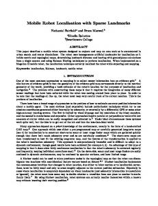
4.1 Active navigation Active navigation was tested by placing the robot in an office environment (see Fig. 1). Notice that the corridor in this environment is basically symmetric and possesses various places that look alike, making it difficult for the robot to determine where it is. In this particular case, the robot must move into one of the offices, since only here it finds distinguishing features.
B
1
2
3
3.4 Efficient Implementation The active navigation and sensing methods described here have been implemented and tested using position probability grids [Burgard et al., 1996]. This technique represents the location of the robot by a discrete three-dimensional grid. To achieve the level of accuracy necessary for predicting robot motion, the resolution of robot orientation is typically in the order of 1� , and the resolution of longitudinal information is often as small as 10cm. While position probability grids are capable of approximating most probability functions of practical interest, they are computationally too expensive for active navigation. The complexity of computing the expected entropy is in O(jLj � jS j), where L denotes the set of grid-cells in the position probability grids, and S the set of distinguishable sensations. For example, for a mid-size environment of size 100m2, jLj = 3; 600; 000 for the resolution specified above. If the number of possible sensations is large, computing the expected entropy is infeasible in real-time. We have modified the basic algorithm in a variety of ways, to ensure all necessary quantities can be approximated in realtime. Most importantly, instead of integrating over all locations L, only a small subset of L is considered, assuming that
A
C
Fig. 1. Environment and path of the robot In a total of 10 experiments, random wandering and/or wall following consistently failed to localize the robot. This is because our wandering routines are highly unlikely to move the robot through narrow doors, and the symmetry of the corridor made it impossible to uniquely determine the location. In more than 20 experiment using the active navigation approach presented here, the robot always managed to localize itself in a considerably short amount of time. Fig. 1 shows a representative example of the path taken during active exploration, and also defines the positions and office names (1, 2, 3, A, B, C) used in the text. In this particular run we started the robot at position 1 in the corridor facing south-west. The task of the robot was to determine its position within the environment, and then to move into room A (so that we could see that localization was successful). After about ten meters of robot motion, it reached position 2 shown in Fig. 1. Fig. 2 depicts the belief Bel(l) at this point
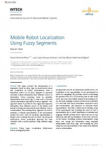
Fig. 3. Occupancy prob. Pocc (a) at pos. 2 Fig. 4. Expected entropy Ea [H] at pos. 2
Fig. 2. Belief Bel(l) at pos. 2 in time (more likely positions are darker). The positions and orientations of the six local maxima are marked by the six circles. The expected occupancy probabilities Pocc(a), obtained by (6), are depicted in Fig. 3. High probabilities are shown in dark colors. Note that this figure roughly corresponds to a weighted overlay of the environmental map relative to the different local maxima, where the weights are given by the probabilities of the local maxima. Fig. 3 also contains the origin of the corresponding coordinate system. In this coordinate system a coordinate hx; yi represents a target point x meters in front of the robot and y meters to the left. Fig. 4 shows the expected entropies of the target points, according to (5). As can be seen there, the expected entropy of locations in rooms is low, making them favorable for localization. It is also low, however, for the two ends of the corridor, since there the uncertainty can be further reduced. Finally, Fig. 5 displays the expected costs for reaching the different target points. (c.f., (7)). Based on the entropy-cost trade-off c.f. (Fig. 6), the robot decided at first to move to the end of the corridor and progressed to position 3. At this point it is important to notice that the trajectory to the target point cannot be computed off-line. This is due to unavoidable inaccuracies in the world model and to unforeseen obstacles in populated environments such as our office. These difficulties are increased if the position of the robot is not known, as is the case during localization. To overcome these problems the robot must be controlled by a reactive collision avoidance technique. In our implementation a global planning module uses dynamic programming as described in section 3.3 to generate a cost minimal path to the target lo-
Fig. 6.
Fig. 5. Expected costs v(a) at pos. 2
Ea[H] + v(a) at pos. 2
cation (see [Thrun and B¨ucken, 1996]). Intermediate target points on this path are sent to our reactive collision avoidance technique described in [Fox et al., 1997]. The collision avoidance then generates motion commands to safely guide the robot to these targets. An overview of the architecture of the navigation system is given in [Buhmann et al., 1995; Thrun et al., to appear].
Fig. 7. Belief Bel(l) at pos. 3 After reaching the end of the corridor (position 3) the belief state contained only two local maxima (see Fig. 7). Note that this kind of ambiguity can no longer be resolved without leaving the corridor. Accordingly the expected entropy of target points in the corridor is high compared to the expected entropy of actions which guide the robot into the rooms. Because of the state of the doors, which only influences the cost of reaching target points, the overall payoff (displayed in Fig. 8) is maximal for target points in rooms B and C. This is why the robot decided to move into the room behind him on the right, which in this case turned out to be room B. After
resolving the ambiguity between the rooms B and C the robot moved straight to the target location in room A. Fig. 9 shows the belief state at this final target point.
passive method was compared to our active approach, where sensors are chosen by minimizing entropy.
active random
14
entropy
12
10
8
6 200
400
600 time
800
1000
Fig. 11. Entropy of belief states Fig. 8.
Ea [H] + v(a) at pos. 3
The results are depicted in Figures 11 and 12. Fig. 11 plots the entropy of Bel(l) as a function of the number of sensor measurements, averaged over 12 runs, along with their variances (bars). As can be seen here, the entropy (uncertainty) decreases much faster when sensors are selected actively. Of course, minimizing entropy alone is not an indicator of successful localization; even a low-entropy estimate could be wrong.
active random
0.4
error
0.3
Fig. 9. Final belief Bel(l) In addition to runs in our real office environment we did extensive testing in simulated hallway environments taken from [Kaelbling et al., 1996]. Our active navigation system successfully localized the robot in every case by automatically detecting junctions of hallways and openings as crucial points for the localization task, and was uniformly superior to passive localization. The exact results are omitted for brevity.
4.2 Active Sensing Our positive results were confirmed in the context of active sensing. Here we placed the robot in the corridor shown in Fig. 10. This corridor ( 23m � 4:5m, all doors closed) is symmetric except for a single obstacle on its side. Thus, to determine its location, the robot has to sense this obstacle.
Fig. 10. Corridor of the department To simulate active sensing, we allowed the robot to read only a single sonar sensor at any point in time. As a passive method, we chose a sensor at random (a new sensor was chosen randomly for every reading, which was the best passive approach out of a number of alternatives that we tried). This
0.2
0.1
200
400
600 time
800
1000
Fig. 12. Estimation error Fig. 12 plots the error in localization (measured by the L1 norm, weighted by Bel(l)) for both approaches as a function of the number of sensor measurements. Here, too, the active approach is more efficient than the passive one. These results demonstrate the benefit of active localization.
5 Conclusions This paper advocates a new, active approach to mobile robot localization. In active localization, the robot controls its various effectors so as to most efficiently localize itself. Based on Markov localization [Burgard et al., 1996; Kaelbling et al., 1996; Nourbakhsh et al., 1995; Simmons and Koenig, 1995; Smith et al., 1990], a popular passive approach to mobile robot localization, this paper describes an approach for determining the robot’s actions during control. In essence, actions are generated by minimizing the future expected uncertainty, measured by entropy. This basic principle has been applied to two active localization problems: active navigation, and active sensing. In the case of active navigation, an extension has been developed that incorporates expected costs into the action selection, and also determines cost-optimal paths under uncertainty using a modified version of dynamic pro-
gramming. Both approaches have been verified empirically using an RWI B21 mobile robot. The key results of our experiments are: 1. The efficiency of localization is increased when actions are selected by minimizing entropy. This is the case for both active navigation and active sensing. In some cases, the active component enabled a robot to localize itself where the passive counterpart failed. 2. The relative advantage of active localization is particularly large if the environment possesses relatively few features that enable a robot to unambiguously determine its location. Despite these encouraging results, there are some limitations that deserve future research. One of the key limitations arises from the algorithmic complexity of the entropy prediction. While a Mixed-Gaussian approximation made the computation of the entropy feasible for the type environments studied here, more research is needed to scale the approach to environments that are significantly larger (e.g., 1000m�1000m). A second limitation arises from the greediness of action selection. In principle, the problem of optimal exploration is NP hard, and there exist situations where greedy solutions will fail. However, in none of our experiments we ever observed that the robot was unable to localize itself using our greedy approach, something that often happens using only random motion during localization.
References [Ballard and Brown, 1982] D.H. Ballard and C.M. Brown. Computer Vision. Prentice-Hall, 1982. [Borenstein et al., 1996] J. Borenstein, B. Everett, and L. Feng. Navigating Mobile Robots: Systems and Techniques. A. K. Peters, Ltd., Wellesley, MA, 1996. [Buhmann et al., 1995] J. Buhmann, W. Burgard, A.B. Cremers, D. Fox, T. Hofmann, F. Schneider, J. Strikos, and S. Thrun. The mobile robot Rhino. AI Magazine, 16(2):31–38, Summer 1995. [Burgard et al., 1996] W. Burgard, D. Fox, D. Hennig, and T. Schmidt. Estimating the absolute position of a mobile robot using position probability grids. In Proc. of the Fourteenth National Conference on Artificial Intelligence, pages 896–901, 1996. [Fox et al., 1997] D. Fox, W. Burgard, and S. Thrun. The dynamic window approach to collision avoidance. IEEE Robotics & Automation Magazine, 4(1):23–33, March 1997. [Kaelbling et al., 1995] L.P. Kaelbling, M.L. Littman, and A.R. Cassandra. Planning and acting in partially observable stochastic domains. Technical report, Brown University, 1995.
[Kaelbling et al., 1996] L.P. Kaelbling, A.R. Cassandra, and J.A. Kurien. Acting under uncertainty: Discrete bayesian models for mobile-robot navigation. In Proc. of the IEEE/RSJ International Conference on Intelligent Robots and Systems, 1996. [Kleinberg, 1994] J. Kleinberg. The localization problem for mobile robots. In Proc. of the 35th IEEE Symposium on Foundations of Computer Science, 1994. [Koenig, 1992] S. Koenig. The complexity of real-time search. Technical Report CMU-CS-92-145, Carnegie Mellon University, April 1992. [Kuipers and Byun, 1981] B. Kuipers and Y.T. Byun. A robot exploration and mapping strategy based on a semantic hierarchy of spatial representations. Robotics and Autonomous Systems, 8 1981. [Littman et al., 1995] M.L. Littman, T.L. Dean, and L.P. Kaelbling. On the complexity of solving markov decision problems. In Proc. of the Eleventh International Conference on Uncertainty in Artificial Intelligence, 1995. [Moravec, 1988] H.P. Moravec. Sensor fusion in certainty grids for mobile robots. AI Magazine, Summer 1988. [Nourbakhsh et al., 1995] I. Nourbakhsh, R. Powers, and S. Birchfield. DERVISH an office-navigating robot. AI Magazine, 16(2), Summer 1995. [Simmons and Koenig, 1995] R. Simmons and S. Koenig. Probabilistic robot navigation in partially observable environments. In Proc. International Joint Conference on Artificial Intelligence, 1995. [Smith et al., 1990] R. Smith, M. Self, and P. Cheeseman. Estimating uncertain spatial realtionships in robotics. In I. Cox and G. Wilfong, editors, Autonomous Robot Vehicles. Springer Verlag, 1990. [Thrun and B¨ucken, 1996] S. Thrun and A. B¨ucken. Integrating grid-based and topological maps for mobile robot navigation. In Proc. of the Fourteenth National Conference on Artificial Intelligence, 1996. [Thrun et al., to appear] S. Thrun, A. B¨ucken, W. Burgard, D. Fox, T. Fr¨ohlinghaus, D. Hennig, T. Hofmann, M. Krell, and T. Schimdt. Map learning and high-speed navigation in RHINO. In D. Kortenkamp, R.P. Bonasso, and R. Murphy, editors, AI-based Mobile Robots: Case studies of successful robot systems. MIT Press, Cambridge, MA, to appear. [Thrun, 1992] S. Thrun. The role of exploration in learning control. In D. A. White and D. A. Sofge, editors, Handbook of intelligent control: neural, fuzzy and adaptive approaches. Van Nostrand Reinhold, Florence, Kentucky 41022, 1992.