Topological Mobile Robot Localization Using Fast Vision Techniques. Paul Blaer and Peter Allen. Department of Computer Science, Columbia University, New ...
Topological Mobile Robot Localization Using Fast Vision Techniques Paul Blaer and Peter Allen Department of Computer Science, Columbia University, New York, NY 10027 {psb15,allen}@cs.columbia.edu
Abstract In this paper we present a system for topologically localizing a mobile robot using color histogram matching of omnidirectional images. The system is intended for use as a navigational tool for the Autonomous Vehicle for Exploration and Navigation of Urban Environments (AVENUE) mobile robot. Our method makes use of omnidirectional images which are acquired from the robot’s on-board camera. The method is fast and rotation invariant. Our tests have indicated that normalized color histograms are best for an outdoor environment while normalization is not required for indoor work. The system quickly narrows down the robot’s location to one or two regions within the much larger test environment. Using this regional localization information, other vision systems that we have developed can further localize the robot.
1
Introduction
The determination of a mobile robot’s location in a complex environment is an interesting and important problem. Localization of the robot can be done geometrically or topologically. In this paper, we present a fast method of topological localization using the analysis of color histograms. Our method can then be used to help another vision system perform precise geometrical localization. This combination of techniques is used to navigate our autonomous site modeling robot AVENUE. The AVENUE project’s [1] overall goal is to automate the site modeling process which includes building geometrically accurate and photometrically correct models of complex outdoor urban environments. These environments are typified by large 3-D structures (i.e. buildings) that encompass a wide range of geometric shapes and a large scope of photometric properties. ∗ This work was supported in part by an ONR/DARPA MURI award ONR N00014-95-1-0601 and NSF grants EIA97-29844 and ANI-0099184.
∗
AVENUE uses a mobile robot platform and a software system architecture that controls the robot to perform human-assisted or fully autonomous data acquisition tasks [7]. For a site modeling task, the robot is provided with a 2-D map of its environment. Highlevel planning software is used to direct the robot to a number of different sensing locations where it can acquire imagery that is fused into a photo-realistic (i.e texture mapped) 3-D model of the site. The system must plan a path to each sensing location and then control the robot to reach that location. Positional accuracy is a paramount concern, since reconstructing the 3-D models requires precise registration among image and range scans from multiple acquisition sites. The navigation portion of the AVENUE system [7] currently localizes the robot through a combination of three different sensor inputs. It makes use of the robot’s built-in odometry, a differential GPS system, and a vision system. The vision system matches edges on nearby buildings with a stored model of those buildings in order to compute the robots exact location. However, to pick the correct building model for comparison, the robot needs to know its approximate location. In urban environments with tall buildings, GPS performance can fail with too few visible satellites. To alleviate this, we have developed a two-level, coarse-fine vision sensing scheme that can supplement GPS and odometry for localization. This paper describes a fast method for topologically locating the robot using vision. Once the robot has been coarsely located in the environment, more accurate vision techniques can be utilized to calculate the exact position and orientation of the robot [6]. The topological location needs to be fast as it works with a set of real-time images which are acquired from the moving mobile robot (see Fig. 1) and which require on-board processing using the mobile robot’s limited computing power. Our method is based upon histogram matching of omnidirectional images acquired from the robot. The method is fast, rotation invariant, and has been tested in both indoor and outdoor environments. It is relatively robust to small
changes in imaging position between stored sample database images and images acquired from unknown locations. As in all histogram methods, it is sensitive to changing lighting conditions. To compensate for this, we have implemented a normalized color space matching metric that improves performance.
2
Related Work
Topological maps for general navigation were originally introduced for use by mobile robots [9]. Many of the methods involve the use of computer vision to detect the transition between regions [12]. Recently a number of researchers have used omnidirectional imaging systems [11] to perform robot localization. Cassinis et al. [2] used omnidirectional imaging for self-localization, but they relied on artificially colored landmarks in the scene. Winters et al. [19] also studied a number of robot navigation techniques utilizing omnidirectional vision. Our work most closely resembles that of Ulrich and Nourbakhsh [17], who originally studied topological localization of a mobile robot using color histograms of omnidirectional images. The primary distinction between the two works is that we address outdoor scenes more thoroughly and we attempt to normalize for variable lighting. The concept of using color histograms as a method of matching two images was pioneered by Swain and Ballard [15]. A number of different metrics for finding the distance between histograms have been explored [8, 14, 18]. Other approaches include simultaneous localization and map building [3, 5, 10, 16], probabilistic approaches [13, 16], and Monte Carlo localization [4].
3
Hardware and Environment
Our mobile robot, AVENUE, has as its base unit the ATRV-2 model manufactured by RWI (see Fig. 1). To this base unit we have added additional sensors including a differential GPS unit, a laser range scanner, two cameras, a digital compass, and wireless Ethernet. The sensor used for our color-histogram localization method is an omnidirectional camera [11] manufactured by Remote Reality. The on-board computer can perform all of the image processing for the method. For our experiments, the robot operated in an indoor and outdoor environment (see Fig. 1). For the indoor environment, we divided the area into
regions corresponding to each of the robot-accessible hallways and rooms. The lighting did not change significantly over time in this environment. The major distinguishing characteristics between regions were the occasional colorful posters on office doors. For the outdoor environment, we divided the area into regions corresponding to which buildings were most prominent. It should be noted that the ground plane around almost all of the buildings had the same brick pattern. Therefore, aiming the omni–camera up (that is, with the mirror facing down at the ground) was not an option, because all of the regions would have looked essentially the same. We needed to aim the camera down in order to obtain a good view of the buildings extending all the way to their tops. This introduced a significant problem with the sun, which would often be visible in the image and would saturate many pixels. We were able to reduce this effect by masking out a large portion of the sky in our images.
4
Vision Processing
The Database: Our method involves building up a database of reference images taken throughout the various known regions that the robot will be exploring at a later time. Each reference image is then reduced to three histograms, using the Red, Green, and Blue color bands. Each histogram has 256 buckets, with each bucket containing the number of pixels in the image with a specific intensity. The location of the pixels in the actual image plays no role in this histogram. When the robot is exploring those same regions at a later time; it will take an image, convert that to a set of three histograms, and attempt to match the histograms against the existing database. The database itself is divided into a set of characteristic regions. The goal is to determine in which specific physical region the robot is currently located. The indoor and outdoor environments have very different lighting and color characteristics, and therefore we have used two different methods of analysis for the histograms. The images themselves, both for the database and for the later unknowns, are taken with the robot’s on-board omnicamera. The images are taken at a resolution of 640x480 with a color depth of 3 bytes per pixel. We use an omnidirectional camera instead of a standard camera because it allows our method to be rotationally invariant. Images taken from the same location but with a different orientation will differ only by a simple rotation. Since the histogram
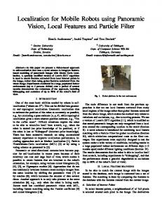
Figure 1: The ATRV-2 Based AVENUE Mobile Robot (left), the outdoor campus environment as seen from above (center) and in outline form (right). only takes into account the colors of the pixels and not their position within the image, two histograms taken from the same location but from a different orientation will essentially be the same. This rotational invariance of the camera allows us to cut down the size of our database considerably, since only one image at a given physical location is needed to get a complete picture of the surrounding area. However, we would still have problems if we were to build our database by driving the robot straight through the center of each region. At different locations in a given region, the proximity of a building or other structure is important. We therefore build up a more comprehensive database by having the robot zigzag through the test environment. This allows us to obtain representative images of a given region from different positions within that region. Although this does increase the size of the database, it is not a major problem because the database is stored as a series of histograms, not images, and the comparison between each of the 256-bucket histograms is very fast. The learning phase of this algorithm, starts with the user inputing which region the robot is about to pass through. At this point the robot starts taking an omni-image once every two seconds. The user drives the robot throughout the region in a zigzag pattern, allowing maximal coverage. As each image is captured by the frame grabber, the training program immediately computes the three color histograms for that particular image. Only the histograms need to be stored, not the images. People walking through the field of view (at a reasonable distance away) have a minimal effect on the histograms.
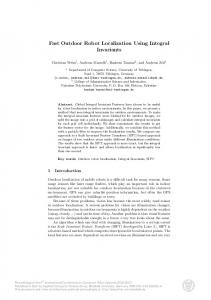
Masking: The histograms are actually constructed only after we have performed some preprocessing on the images. Unwanted portions of the omni-image must be eliminated. First, we only consider pixels within the circular mirror and ignore the outer pixels resulting from the tube which surrounds the optical equipment. We do this by finding the center and radius of the mirror in the image and then ignoring all pixels outside that circle (see Fig. 2). Second, there are fixed pieces of the robot’s superstructure that are always present and always in the same orientation (since these pieces and the camera are attached to the robot and never move with respect to each other). We create a bit-map mask, mark all of the pixels that lie on the robot’s superstructure, and apply that mask to each image that we take. This way we only concentrate on the pixels that should be different from image to image. Finally, we need to eliminate the camera itself from the omni-image. This is done in a manner similar to our handling of the unwanted outer pixels. We take the center and the radius of the camera in the image, and exclude all pixels inside the corresponding circle. Because our camera was positioned to look straight up at the sky and because the sky can vary greatly in color, we also needed some way to minimize the amount of sky visible. Instead of having the inner pixel mask just cover the camera, we extended it out even further to block out much of the sky. However, if we were to enlarge this mask too much, we would cut off much of the surrounding buildings. These buildings are in fact a key feature for our algorithm because they often are of different colors. By experimenting with different
Figure 2: Outdoor Omni-Image Unmasked (top left), Masked (top center), Indoor Omni-Image Unmasked (top right), Unwarped Outdoor Omni-Image (bottom). mask radii, we were able to find a reasonable compromise mask size which eliminated much of the sky without significantly cutting off the tops of buildings. Environmental Effects: The controlled lighting environment of the indoor regions cannot be duplicated in our outdoor tests even with the most cooperative weather conditions. In order to reduce variation as much as possible, we used a normalization process on the images before histograming them. This proG B R , R+G+B , and R+G+B of each given cess uses R+G+B pixel for the histograming. This gives us the percentage of each color at that particular pixel regardless of the overall intensity of that pixel. So, in theory, for a fixed physical location, if a pixel of a certain color was highly illuminated in one image and was in a slight shadow in another image, there should be the same percentages of each color after normalization in both images. In the indoor environments, we could use either the normalized or the non-normalized images because of the low variation in lighting conditions. We chose the normalized images for use in the highly variable outdoor images. Matching: At this point, our software has a collection of histograms grouped together according to their region. We can now use this database to try to match an unknown image to it and find the proper region for this unknown. When we initially compare two histograms together, we treat each color band separately. Going through bucket by bucket, we compute the absolute value of the difference between the two histograms at that particular bucket and then sum these differences across all buckets. This metric measures the difference between the two histograms
in each of the red, green, and blue bands. Experimentally, we find that taking the sum of the three differences across the color bands gives a much better indicator than any one of the color bands taken by itself. To find the reference region that corresponds to an unknown image, we histogram the unknown image and use our metric to determine the difference between it and each of the histograms stored in our database. We then pick the histogram with the smallest difference in each of the regions in our database. Of these smallest differences, we then pick the very smallest and choose the region of that known reference histogram as the region for the unknown. This method allows us to find the region with the absolute minimum histogram difference, but it also permits us to identify those regions whose histograms have a difference which is within a certain range of the absolute minimum. By reducing the number of possible regions, we can more effectively search for a precise location using more exact vision methods (see the discussion in section 6).
5
Experiments
In figure 4, a typical set of normalized and nonnormalized histograms in the three color bands is shown for an outdoor image. We built a reference database of images which were obtained from the robotics laboratory and from the other offices and hallways on our floor. There were 12 distinct regions, each with an approximately equal
Region 1 2 3 4 5 6 7 8 Total
Images Tested 21 12 9 5 23 9 5 5 89
Non-Normalized % Correct 100% 83 % 77% 20% 74% 89% 0% 100% 78%
Normalized % Correct 95% 92% 89% 20% 91% 78% 20% 40% 80%
Region 1 2 3 4 5 6 7 8 Total
Images Tested 50 50 50 50 50 50 50 50 400
Non-Normalized % Correct 58% 11% 29% 25% 49% 30% 28% 41% 34%
Normalized % Correct 95% 39% 71% 62% 55% 57% 61% 78% 65%
Figure 3: Results of an indoor test (left). Test images were taken from only 8 of 12 regions. Results of an outdoor test (right). Test images were taken from all 8 regions. 30000 "normal.hist.red" "normal.hist.green" "normal.hist.blue" "notnormal.hist.red" "notnormal.hist.green" "notnormal.hist.blue"
25000
Number of Pixels
20000
15000
10000
5000
0 0
50
100
150
200
250
Intensity
Figure 4: The normalized and non-normalized histograms of a typical masked outdoor omni-image.
number of images (50) in them. We created two versions of this database, one normalized and one nonnormalized. All images had the necessary masking. We then took a second set of images throughout our indoor region to be used as unknowns. When the nonnormalized unknown images were compared against the non-normalized database, we obtained an overall success rate of 78% (see Fig. 3). When utilizing the normalized database with normalized unknowns, we obtained a success rate of 80% (see Fig. 3). The success rate was consistently good throughout the indoor regions with the exceptions of regions 4 and 7. These two regions are in fact located at the corners of the hallways. They are small transition areas between two much larger and more distinctive regions, and they are also extremely similar to each other. For these reasons, our algorithm had difficulty distinguishing the two regions from each other and from the larger regions on which they bordered.
We repeated the same test on a set of outdoor regions that spanned the northern half of the Columbia campus. There were 8 distinct regions in this test, and each of these regions had approximately 120 images. We again created two versions of the database, one normalized and one non-normalized. We then took a second set of outdoor images to be used as unknowns. When using non-normalized images for the histograms, we achieved a success rate of 34% (see Fig. 3). When using normalized images, the success rate was increased to 65% (see Fig. 3). The majority of the regions had consistently good success percentages, with the exception of region 2. This region was a very special case because one of the large buildings which dominated a different region (region 1) was still prominently visible when the robot was in region 2. However, the two regions were at a large enough physical distance apart that it would not have been appropriate to consider them a single region. Using the set of outdoor unknowns, we also computed all of the regions whose histogram differences were within 10% of the minimum histogram difference. In most cases there were only two other regions that fell within this range, and 80% of the time one of those regions was the correct one.
6
Summary and Future Work
When we performed our matching tests with the indoor database, we found that the difference between the results of using non-normalized images versus normalized images was not significant. The success rate for the normalized ones was 80%, only about 2% better than for the non-normalized. When we performed our database matching tests outdoors, the normalized images had a success rate that was about twice as high as the non-normalized. This was what we
were expecting. However, the success rates were still noticeably lower outdoors than indoors. The normalized outdoor images gave us success rates of about 65%. There was however a very helpful feature. We could identify a small number of regions whose histograms were close to the best-matched histogram. This reliably narrowed down the possible regions for the robot from 8 to 2 or 3. The color histogram method described in this paper is part of the larger AVENUE project, which contains another vision based localization system. This other localization method matches images of the facades of nearby buildings with pre-existing models of those buildings. From these matches, exact information on the position of the robot can be found [6]. However, this system assumes that we have some previous information as to where in the environment the robot actually is. Using previous, presumably accurate, odometry and GPS data, it then attempts to match the robot’s environment with models of buildings that should be nearby. However, one can not always make the assumption that the GPS data or odometry data is that good. In particular, when the robot is very near buildings, GPS data is virtually useless. The algorithm presented in this paper can narrow down the general location to within two or three possibilities. This greatly decreases the number of models against which the main vision system has to attempt a match. The combination of the two systems will allow us to accurately localize our robot within its test environment without any artificial land marks or pre-existing knowledge about its position. What is needed next is a fast secondary discriminator to distinguish between the two or three possible regions to further decrease the work load of the main vision system. One possibility would be to record the robot’s initial region and then keep track of the regions already passed, thus narrowing down the possibilities for the next region. We also plan to add the use of edge images to the system so that we can encode some geometric information into our database that will be independent of the lighting of the scene. A metric based on the edge images could then be used as a secondary discriminator on the narrowed-down possibilities resulting from the algorithm presented in this paper.
References [1] P. K. Allen, I. Stamos, A. Gueorguiev, E. Gold, and P. Blaer. Avenue: Automated site modeling in urban environments. In 3DIM, Quebec City, pages 357–364, May 2001.
[2] R. Cassinis, D. Grana, and A. Rizzi. Self-localization using an omni-directional image sensor. In International Symposium on Intelligent Robotic Systems, pages 215– 222, July 1996. [3] J. A. Castellanos, J. M. Martinez, J. Neira, and J. D. Tardos. Simultaneous map building and localization for mobile robots: A multisensor fusion approach. In IEEE ICRA, pages 1244–1249, 1998. [4] F. Dellaert, D. Fox, W. Burgard, and S. Thrun. Monte Carlo localization for mobile robots. In IEEE ICRA, pages 1322–1328, 1999. [5] H. Durrant-Whyte, M. Dissanayake, and P. Gibbens. Toward deployment of large scale simultaneous localization and map building (SLAM) systems. In Proc. of Int. Simp. on Robotics Research, pages 121–127, 1999. [6] A. Georgiev and P. K. Allen. Vision for mobile robot localization in urban environments. Submitted to IEEE IROS, 2002. http://www.cs.columbia.edu/∼atanas/research/ iros02/iros02.pdf. [7] A. Gueorguiev, P. K. Allen, E. Gold, and P. Blaer. Design, architecture and control of a mobile site modeling robot. In IEEE ICRA, pages 3266–3271, April 24-28 2000. [8] J. Hafner and H. S. Sawhney. Efficient color histogram indexing for quadratic form distance functions. IEEE PAMI, 17(7):729–735, July 1995. [9] B. Kuipers and Y.-T. Byun. A robot exploration and mapping strategy based on a semantic hierarchy of spatial representations. Journal of Robotics and Autonomous Systems, 8:47–63, 1991. [10] J. Leonard and H. J. S. Feder. A computationally efficient method for large-scale concurrent mapping and localization. In Proc. of Int. Simp. on Robotics Research, pages 128–135, 1999. [11] S. Nayar. Omnidirectional video camera. In Proc. DARPA IUW, pages 235–242, May 12-14 1997. [12] D. Radhakrishnan and I. Nourbakhsh. Topological robot localization by training a vision-based transition detector. In IEEE IROS, pages 468–473, October 1999. [13] R. Simmons and S. Koenig. Probabilistic robot navigation in partially observable environments. In IJCAI, pages 1080–1087, 1995. [14] M. Stricker and M. Orengo. Similarity of color images. In SPIE Conference on Storage and Retrieval for Image and Video Databases III, volume 2420, pages 381–392, February 1995. [15] M. Swain and D. Ballard. Color indexing. International Journal of Computer Vision, 7(1):11–32, 1991. [16] S. Thrun, W. Burgard, and D. Fox. A probabilistic approach to concurrent mapping and localization for mobile robots. Autonomous Robots, 5:253–271, 1998. [17] I. Ulrich and I. Nourbakhsh. Appearance-based recognition for topological localization. In IEEE ICRA, pages 1023–1029, April 24-28 2000. [18] M. Werman, S. Peleg, and A. Rosenfeld. A distance metric for multi-dimensional histograms. In CVGP, volume 32, pages 328–336. 1985. [19] N. Winters, J. Gaspar, G. Lacey, and J. Santos-Victor. Omni-directional vision for robot navigation. In IEEE Workshop on Omnidirectional Vision, pages 21–28, June 12 2000.