Paul J. Besl. Computer Science ..... This sen- sor features an auto-calibration feature that cali- brates the system every frame avoiding thermal drift problems ...
Machine Vision and Applications (1988) 1:127-152
Machine Vision and Applications 9 1988 Springer-VerlagNew York Inc.
Active, Optical Range Imaging Sensors Paul J. Besl Computer Science Department, General Motors Research Laboratories, Warren, Michigan 48090-9055 USA
Abstract: Active, optical range imaging sensors collect three-dimensional coordinate data from object surfaces and can be useful in a wide variety of automation applications, including shape acquisition, bin picking, assembly, inspection, gaging, robot navigation, medical diagnosis, and cartography. They are unique imaging devices in that the image data points explicitly represent scene surface geometry in a sampled form. At least six different optical principles have been used to actively obtain range images: (1) radar, (2) triangulation, (3) moire, (4) holographic interferometry, (5) focusing, and (6) diffraction. In this survey, the relative capabilities of different sensors and sensing methods are evaluated using a figure of merit based on range accuracy, depth of field, and image acquisition time.
Key Words: range image, depth map, optical measurement, laser radar, active triangulation
1.
Introduction
Range-imaging sensors collect large amounts of three-dimensional (3-D) coordinate data from visible surfaces in a scene and can be used in a wide variety of automation applications, including object shape acquisition, bin picking, robotic assembly, inspection, gaging, mobile robot navigation, automated cartography, and medical diagnosis (biostereometrics). They are unique imaging devices in that the image data points explicitly represent scene surface geometry as sampled points. The inherent problems of interpreting 3-D structure in other types of imagery are not encountered in range imagery although most low-level problems, such as filtering, segmentation, and edge detection, remain. Most active optical techniques for obtaining range images are based on one of six principles: (1) radar, (2) triangulation, (3) moire, (4) holographic interferometry, (5) lens focus, and (6) Fresnel diffraction. This paper addresses each fundamental category by discussing example sensors from that
class. To make comparisons between different sensors and sensing techniques, a performance figure of merit is defined and computed for each representative sensor if information was available. 'This measure combines image acquisition speed, depth of field, and range accuracy into a single number. Other application-specific factors, such as sensor cost, field of view, and standoff distance are not compared. No claims are made regarding the completeness of this survey, and the inclusion of commercial sensors should not be interpreted in any way as an endorsement of a vendor's product. Moreover, if the figure of merit ranks one sensor better than another, this does not necessarily mean that it is better than the other for any given application. Jarvis (1983b) wrote a survey of range-imaging methods that has served as a classic reference in range imaging for computer vision researchers. An earlier survey was done by Kanade and Asada (1981). Strand (1983) covered range imaging techniques from an optical engineering viewpoint. Several other surveys have appeared since then (Kak 1985, Nitzan et al. 1986, Svetkoff 1986, Wagner 1987). The goal of this survey is different from previous work in that it provides a simple example methodology for quantitative performance comparisons between different sensing methods which may assist system engineers in performing evaluations. In addition, the state of the art in range imaging advanced rapidly in the past few years and is not adequately documented elsewhere. This survey is structured as follows. Definitions of range images and range-imaging sensors are given first. Different forms of range images and generic viewing constraints and motion requirements are discussed next followed by an introduction to sensor performance parameters, which are then used to define a figure of merit. The main body sequentially addresses each fundamental ranging method. The figure of merit is computed for each sensor if possible. The conclusion consists of a sen-
128
Besl: Range Imaging Sensors
sor comparison section and a final summary. An introduction to laser eye safety is included in the appendix. This paper is an abridged version of Besl (1988), which was derived from sections of Besl (1987). Tutorial material on range-imaging techniques may be found in both as well as in the references.
2.
the sampling intervals are consistent in the x- and y-directions of an x y z range image, it can be represented in the form of a large matrix of scaled, quantized range values r~/where the corresponding x, y, z coordinates are determined implicitly by the row and column position in the matrix and the range value. The term "image" is used because any rii range image can be displayed on a video monitor, and it is identical in form to a digitized video image from a TV camera. The only difference is that pixel values represent distance in a range image whereas they represent irradiance (brightness) in a video image. The term "large" in the definition above is relative, but for this survey, a range image must specify more than 100 (x, y, z) sample points. In Figure 1, the 20 x 20 matrix of heights of surface points above a plane is a small range image. If rij is the pixel value at the ith row and the flh column of the matrix, then the 3-D coordinates would be given as
Preliminaries
A r a n g e - i m a g i n g s e n s o r is any combination of hardware and software capable of producing a r a n g e i m a g e of a real-world scene under appropriate operating conditions. A range i m a g e is a large collection of distance m e a s u r e m e n t s from a known reference coordinate system to s u r f a c e p o i n t s on object(s) in a scene. If scenes are defined as collections of physical objects and if each o b j e c t is defined by its mass density function, then surface points are defined as the 3-D points in the halfdensity level set of each object's normalized massdensity function as in Koenderink and VanDoorn (1986). Range images are known by many other names depending on context: range map, depth map, depth image, range picture, rangepic, 3-D image, 2.5-D image, digital terrain map (DTM), topographic map, 2.5-D primal sketch, surface profiles, x y z point list, contour map, and surface height map. If the distance measurements in a range image are listed relative to three orthogonal coordinate axes, the range image is in x y z form. If the distance measurements indicate range along 3-D direction vectors indexed by two integers (i, J), the range image is in r~/form. Any range image in r;j form can be converted directly to x y z form, but the converse is not true. Since no ordering of points is required in the x y z form, this is the more general form, but it can be more difficult to process than the rij form. If 171 168 168 166 163 166 163 160 163 166 167 167 167 167 157 168 162 lS6 166 166
160 165 168 163 166 163 166 160 166 160 186 167 160 165 167 167 167 166 167 166
163 166 166 166 160 1G3 166 leo 167 160 163 166 166 160 157 160 166 167 162 166
163 163 166 166 166 163 187 166 163 163 160 167 16S 160 160 160 186 162 167 16E
166 166 166 163 163 168 160 167 160 160 167 160 167 167 157 160 152 162 149 182
166 163 163 163 163 160 160 160 167 163 lS? 167 167 157 167 162 166 166 167 149
168 168 160 160 166 163 160 168 160 160 168 163 168 163 162 166 lt9 156 167 lt6
166 166 166 163 190 166 171 166 177 166 166 171 168 157 166 182 163 171 168 174
168 166 166 179 l?t 166 160 166 166 166 168 163 163 167 160 163 160 l?t 179 188
166 166 171 174 168 163 168 163 160 163 163 167 166 160 163 162 166 166 204 193
163 163 166 186 168 168 1e8 1G$ 171 163 177 166 166 157 166 168 187 171 182 168
160 163 158 177 182 177 182 182 201 20t 188 20t 1gO 182 193 171 188 188 221 la6
163 166 168 186 186 190 199 201 216 207 201 186 201 204 196 212 210 188 l?t 168
163 163 166 179 190 188 199 199 199 207 199 196 201 190 193 212 210 199 193 179
x = ax + Sxi
y
= ay +
Syj
Z = az + Szro (1)
where the Sx, Sy, Sz values are scale factors and the a x, a y , a z values are coordinate offsets. This matrix of numbers is plotted as a surface viewed obliquely in Figure 2, interpolated and plotted as a contour map in Figure 3, and displayed as a black and white image in Figure 4. Each representation is an equally valid way to look at the data. The affine transformation in equation (1) is appropriate for orthographic r o. range images where depths are measured along parallel rays orthogonal to the image plane. Nonaffine transformations of (i, j, ro.) coordinates to Cartesian (x, y, z) coordinates are more common in active optical range sensors. In the spherical coordinate system shown in Figure 160 166 160 212 201 199 199 190 lg6 190 196 193 196 186 199 193 212 188 182 171
163 163 163 196 196 188 193 188 201 188 196 188 188 190 190 190 216 20t 179 190
166 166 166 186 199 190 199 190 190 193 201 196 190 190 190 188 210 188 212 190
163 160 160 20t 182 196 188 190 1go 190 182 188 193 188 186 182 186 186 188 193
166 163 160 196 196 193 193 193 188 196 210 193 186 186 190 188 204 216 201 190
163 163 166 186 199 186 193 193 188 196 196 201 193 188 186 186 193 207 182 179
Figure 1. 20 • 20 matrix of range measurements: r~j form of range image.
Besl: Range Imaging Sensors
129
spherical azimuth definition 0. The transformation to Cartesian coordinates is X = a x + Srr U
tan(jso)/~v/1 + tanZ(iso) + tan2(js,)
(3)
y = ay + Srrij tan(is+)/~v/1 + tan2(iso) + tan2(js+) z = az + s,.ro'/'~v/1 + tanZ(iso) + tanZ(/s+).
The alternate elevation angle t~ depends only on y and z whereas + depends on x, y, and z. The differences in (x, y, z) for equations (2) and (3) for the same values of azimuth and elevation are less than 4% in x and z and less than 11% in y, even when both angles are as large as -+30 degrees. 2.1
Figure 2. Surface plot of range image in Figure 1. 5, the (i, j) indices correspond to elevation (latitude) angles and azimuth (longitude) angles respectively. The spherical to Cartesian transformation is x = ax + Srro cos(is+)sin(jso)
(2)
y = ay + Srrij sin(is+) z = az + Srr O Cos(is+)cos(jso)
where the st, s+, so values are the scale factors in range, elevation, and azimuth and the ax, ay, a z values are again the offsets. The "orthogonal-axis" angular coordinate system, also shown in Figure 5, uses an "alternate elevation angle" + with the
Figure 3. Contour plot of range image in Figure 1.
Viewing Constraints and
Motion Requirements The first question in range imaging requirements is v i e w i n g c o n s t r a i n t s . Is a single view sufficient, or are multiple views of a scene necessary for the given application? What types of sensors are compatible with these needs? For example, a mobile robot can acquire data from its on-board sensors only at its current location. An automated modeling system may acquire multiple views of an object with many sensors located at different viewpoints. Four basic types of range sensors are distinguished based on the viewing constraints, scanning mechanisms, and object movement possibilities: I. A P o i n t S e n s o r measures the distance to a single visible surface point from a single viewpoint along a single ray. A point sensor can create a range image if (1) the scene object(s) can be physically moved in two directions in front of the point-ranging sensor, (2) if the point-ranging sensor can be scanned in two directions over the scene, or (3) the scene object(s) are stepped in
Figure 4. Gray level representation of range image in Figure l.
130
Besl: Range Imaging Sensors
one direction while the point sensor is scanned in the other direction. 2. A Line or Circle Sensor measures the distance to visible surface points that lie in a single 3-D plane or cone that contains the single viewpoint or viewing direction. A line or circle sensor can create a range image if (1) the scene object(s) can be moved orthogonal to the sensing plane or cone or (2) the line or circle sensor can be scanned over the scene in the orthogonal direction. 3. A Field o f View Sensor measures the distance to many visible surface points that lie within a given field of view relative to a single viewpoint or viewing direction. This type of sensor creates a range image directly. No scene motion is required. 4. A Multiple View Sensor System locates surface points relative to more than one viewpoint or viewing direction because all surface points of interest are not visible or cannot be adequately measured from a single viewpoint or viewing direction. Scene motion is not required. These sensor types form a natural hierarchy: a point sensor may be scanned (with respect to one sensor axis) to create a line or circle sensor, and a line or circle sensor may be scanned (with respect to the orthogonal sensor axis) to create a field of view sensor. Any combination of point, line/circle, and field of view sensors can be used to create a multiple view sensor by (1) rotating and/or translating the scene in front of the sensor(s); (2) maneuvering the sensor(s) around the scene with a robot; (3) using multiple sensors in different locations to capture the appropriate views; or any combination of the above. Accurate sensor and/or scene object positioning is achieved via commercially available translation stages, xy(z)-tables, and xy0 tables (translation repeatability in submicron range, angular repeatabilPoint
Alternate Elevation Angle~ / ~
~-/ ~ ~
z/ Azimuth Angle 0
Elevation Angle ,~
Sensor
Origin Figure 5. Cartesian, spherical, and orthogonal-axis coordinates.
ity in microradians or arc-seconds). Such methods are preferred to mirror scanning methods for high precision applications because these mechanisms can be controlled better than scanning mirrors. Controlled 3-D motion of sensor(s) and/or object(s) via gantry, slider, and/or revolute joint robot arms is also possible, but is generally much more expensive than table motion for the same accuracy. Scanning motion internal to sensor housings is usually rotational (using a rotating mirror), but may also be translational (using a precision translation stage). Optical scanning of lasers has been achieved via (1) motor-driven rotating polygon mirrors, (2) galvanometer-driven flat mirrors, (3) acoustooptic (AO) modulators, (4) rotating holographic scanners, or (5) stepper-motor-driven mirrors (Gottlieb 1983, Marshall 1985). However, AO modulators and holographic scanners significantly attenuate laser power, and AO modulators have a narrow angular field of view (~10 ~ x 10~ making them less desirable for many applications. 2.2 Sensor Performance Parameters Any measuring device is characterized by its measurement resolution or precision, repeatability, and accuracy. The following definitions are adopted here. Range resolution or range precision is the smallest change in range that a sensor can report. Range repeatability refers to statistical variations as a sensor makes repeated measurements of the exact same distance. Range accuracy refers to statistical variations as a sensor makes repeated measurements of a known true value. Accuracy should indicate the largest expected deviation of a measurement from the true value under normal operating conditions. Since range sensors can improve acc u r a c y by averaging multiple m e a s u r e m e n t s , accuracy should be quoted with measurement time. For our comparisons, a range sensor is characterized by its accuracy over a given measurement interval (the depth of field) and the measurement time. If a sensor has good repeatability, we assume that it is also calibrated to be accurate. Loss of calibration over time (drift) is a big problem for poorly engineered sensors but is not addressed here. A range-imaging sensor measures point positions (x, y, z) within a specified accuracy or error tolerance. The method of specifying accuracy varies in different applications, but an accuracy specification should include one or more of the following for each 3-D direction given N observations: (1) the mean absolute error (MAE) (---~x, ---By, ---8z) where 8x = (1/N)~lx;- ~xl and txx = (1/N)'Zxi (or tx~ = median (xi)); (2) RMS (root-mean-square) error (+--trx, -+try, -O'z) where 0-2 = (N - 1)-l~(x i - i~x)2 and I~ =
Besl: Range Imaging Sensors
(1/N)Exi; or (3) maximum error (___ex, "t-Ey, -----EZ) where ex = maxilxi - IXxl. (Regardless of the measurement error probability distribution, g