Hindawi Publishing Corporation Mathematical Problems in Engineering Volume 2014, Article ID 905108, 6 pages http://dx.doi.org/10.1155/2014/905108
Research Article Active Power Measurement Based on Multiwavelet Transforms Xiao-Bing Zhang, Yun-Hui Li, and Xiao-Meng Cui School of Measurement and Communication, Harbin University of Science and Technology, Harbin 150080, China Correspondence should be addressed to Xiao-Bing Zhang; zhangxb
[email protected] Received 29 June 2013; Revised 31 December 2013; Accepted 2 January 2014; Published 11 February 2014 Academic Editor: Claudio R. Fuerte-Esquivel Copyright © 2014 Xiao-Bing Zhang et al. This is an open access article distributed under the Creative Commons Attribution License, which permits unrestricted use, distribution, and reproduction in any medium, provided the original work is properly cited. This paper discusses a new method for calculating active power in the multiwavelet domain. When the voltage and current waveforms are analyzed using multiwavelet, the active power can be calculated by simply adding the products of the multiwavelet coefficients without having to reconstruct the signals back to the time domain first and then using the traditional integration. From the simulation result, we can see that the results using multiwavelet are better than the ones using wavelet and Fourier Transforms no matter which prefilter is used.
1. Introduction
2. Multiwavelet Transform
Active power is important for many purposes such as designing power system equipment, setting tariffs, developing measurement meters, and designing compensation devices for improving the quality of the electric energy. Under sinusoidal conditions, the definitions of active power work well. However, due to the recent widespread use of nonlinear loads, the voltage and current waveforms become nonsinusoidal and therefore their traditional definitions become unsuitable. As a result, many attempts have been made to define active power under this new situation [1–5]. Wavelet is an effective tool for nonstational signal processing and has been used in the measurement of active power [6–8]. However, scalar wavelets cannot contain orthogonality, symmetry, compact support, and higher order of vanishing moments simultaneously. Multiwavelet transform is a new concept in the framework of wavelet transform but has some important differences. It simultaneously possesses orthogonality, compact support, higher order of vanishing moments, and symmetry. It has become a tool for power quality study recently [9–11]. In this paper, a new approach to measure active power based on multiwavelet transforms is studied. In Section 2, we introduce the multiwavelet transform. In Section 3, a new approach to measure active power based on multiwavelet transforms is discussed. In Section 4, an example is given to illustrate validity of our method. At last a conclusion is given in Section 5.
Unlike a scalar wavelet, a multiwavelet has several mother wavelet functions (scaling functions) which are used to expand a given function [12]. Let Φ denote a compactly supported orthonormal scaling vector Φ = (𝜙1 , . . . , 𝜙𝑟 )𝑇 , where 𝑟 is the number of scalar scaling functions. Then Φ(𝑡) satisfies a two-scaling dilation equation of the form Φ (𝑡) = ∑𝐻𝑘 Φ (2𝑡 − 𝑘) 𝑘
(1)
for some finite sequence 𝐻 of 𝑟×𝑟 matrices. Furthermore, the integer shifts of the components of Φ form an orthonormal system; that is, ⟨𝜙𝑛 (⋅ − 𝑘) , 𝜙𝑛 (⋅ − 𝑘 )⟩ = 𝛿𝑛−𝑛 ,𝑘−𝑘 .
(2)
Let 𝑉0 denote the closed span of {𝜙𝑛 (⋅ − 𝑘) | 𝑘 ∈ Z, 𝑛 = 1, 2, . . . , 𝑟} and define 𝑉𝑗 = {𝑓(2𝑗 ⋅) | 𝑓 ∈ 𝑉0 }. Then (𝑉𝑗 )𝑗∈Z is a multiresolution analysis of 𝐿2 (R) [13]. Note that we choose the increasing convention 𝑉𝑗−1 ⊂ 𝑉𝑗 . Let 𝑊𝑗 denote the orthogonal complement of 𝑉𝑗 in 𝑉𝑗+1 . Then there exists an orthogonal multiwavelet Ψ = (𝜓1 , . . . , 𝜓𝑟 )𝑇 such that {𝜓𝑛 (⋅ − 𝑘) | 𝑛 = 1, 2, . . . , 𝑟 and 𝑘 ∈ Z} forms an orthogonal basis of 𝑊0 . Since 𝑊0 ⊂ 𝑉1 , there exists a sequence 𝐺 of 𝑟 × 𝑟 matrices such that Ψ (𝑡) = ∑𝐺𝑘 Φ (2𝑡 − 𝑘) . 𝑘
(3)
2
Mathematical Problems in Engineering
Let 𝑓 ∈ 𝑉0 ; then 𝑓 can be written as a linear combination of the basis in 𝑉0 . Consider 𝑓 (𝑡) = ∑ c∗0 (𝑘) Φ (𝑡 − 𝑘)
(4)
𝑘∈Z
for some sequence c0 ∈ 𝑙2 (Z)𝑟 of vector coefficients. The superscript ∗ stands for the complex conjugate transposition. Here 𝑙2 (Z)𝑟 denotes the space of finite energy vector sequences c with the norm 1/2
2 ‖c‖ = ( ∑ c𝑖 (𝑛) )
.
(5)
𝑖=1,...,𝑟 𝑛∈Z
Because 𝑉0 = 𝑉−1 ⊕ 𝑊−1 [14], where the symbol ⊕ denotes an orthogonal direct sum, 𝑓 can be written as a linear combination of the basis functions of 𝑉−1 and 𝑊−1 𝑓 (𝑡) = ∑ √2c∗1 (𝑘) Φ (2𝑡 − 𝑘) + ∑ √2d∗1 (𝑘) Ψ (2𝑡 − 𝑘) . 𝑘∈Z
𝑘∈Z
(6) The coefficients c1 and d1 are related to c0 via the following decomposition and reconstruction algorithm: c1 (𝑘) = ∑𝐻 (𝑛) c0 (2𝑘 + 𝑛) ,
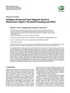
Multiwavelets are a new addition to the body of wavelet theory. Realizable as matrix-valued filter banks leading to wavelet bases, multiwavelets offer simultaneous orthogonality, symmetry, and short support, which is not possible with scalar two-channel wavelet systems. The DGHM multiwavelets which are developed by Donovan et al. [15] are a very popular multiwavelet. They are shown in Figure 1. Remark 1. It is important to note that the orthogonality conditions for the DGHM scaling function and the associated multiwavelet remain valid even when restricted to a compact interval. This is not true in general. It is actually another favorable property of this multiwavelet system. The DGHM scaling functions satisfy (1) with four coefficients: 2√2 3 10 5 ), 𝐻0 = ( √2 3 − − 40 20
3 0 10 ), 𝐻1 = ( 9√2 1 40 2
0
0
0
𝐻2 = ( √ ), 9 2 3 − 40 20
(12)
0
𝐻3 = ( √ ). 2 − 0 40
𝑛
d1 (𝑘) = ∑𝐺 (𝑛) c0 (2𝑘 + 𝑛) ,
(7)
𝑛
c0 (𝑘) = ∑𝐻∗ (𝑘 − 2𝑛) c1 (𝑛) + ∑𝐺∗ (𝑘 − 2𝑛) d1 (𝑛) . 𝑛
Define Φ𝑙,𝑘 (𝑡) = 2𝑙/2 Φ(2𝑙 𝑡 − 𝑘) and Ψ𝑙,𝑘 (𝑡) = 2𝑙/2 Ψ(2𝑙 𝑡 − 𝑘); then {Φ𝑙,𝑘 : 𝑘 ∈ Z} and {Ψ𝑙,𝑘 : 𝑘 ∈ Z} are stable bases of 𝑉𝑙 and 𝑊𝑙 , respectively. And (6) can be written as 𝑓 (𝑡) =
(𝑘) Φ1,𝑘 (𝑡) +
∑ d∗1 𝑘∈Z
(𝑘) Ψ1,𝑘 (𝑡) .
(8)
Because 𝑉0 = 𝑉−1 ⊕𝑊−1 = (𝑉−2 ⊕ 𝑊−2 ) ⊕ 𝑊−1 = ⋅ ⋅ ⋅ = 𝑉−𝑚 ⊕𝑊−𝑚 ⊕⋅ ⋅ ⋅⊕𝑊−1 , where 𝑚 is the levels for decomposition, 𝑓 can be written as 𝑓 (𝑡) =
∑ c∗𝑚 𝑘∈Z
(𝑘) Φ𝑚,𝑘 (𝑡) +
−1
∑ ∑ d∗𝑙 𝑙=−𝑚 𝑘∈Z
(𝑘) Ψ𝑙,𝑘 (𝑡) .
(9)
In general, for a signal 𝑓(𝑡) ∈ 𝑉𝑛 , 𝑛 ∈ Z, it can be expressed as a linear combination of the basis in 𝑉𝑛 . Consider 𝑓 (𝑡) = ∑c∗𝑛 (𝑘) Φ𝑛,𝑘 (𝑡) .
(10)
𝑘
√2 40
3 40 ), 𝐺0 = ( 1 3√2 − − 20 20 −
𝑛
∑ c∗1 𝑘∈Z
And the multiwavelets satisfy (1) with four coefficients as
−
9√2 3 − 40 20 ), 𝐺2 = ( 9 3√2 − 20 20
9√2 1 − 2) , 𝐺1 = ( 40 9 0 20 √2 − 0 𝐺3 = ( 40 ) . 1 0 20
(13)
GHM multiple scaling functions and multiwavelets are very popular with many advantages over scalars. They are either symmetric or antisymmetric, orthogonal, supported on [0, 1] and [0, 2], respectively, with approximation order 2. However, it is impossible for scalar wavelets [16]. Let c𝑗 (𝑘) = (𝑐1,𝑗,𝑘 , 𝑐2,𝑗,𝑘 ) and d𝑗 (𝑘) = (𝑑1,𝑗,𝑘 , 𝑑2,𝑗,𝑘 ). By dilations (1) and (3), we have the following recursive relationship between the coefficients (𝑐1,𝑗,𝑘 , 𝑐2,𝑗,𝑘 )𝑇 and (𝑑1,𝑗,𝑘 , 𝑑2,𝑗,𝑘 )𝑇 :
Similar to (9), 𝑛−1
𝑓 (𝑡) = ∑c∗𝑙 (𝑘) Φ𝑙,𝑘 (𝑡) + ∑ ∑d∗𝑗 (𝑘) Ψ𝑗,𝑘 (𝑡) , 𝑘
(11)
(
𝑐1,𝑗−1,𝑘 𝑐 ) = ∑𝐻𝑛−2𝑘 ( 1,𝑗,𝑛 ) , 𝑐2,𝑗−1,𝑘 𝑐2,𝑗,𝑛 𝑛
𝑗, 𝑘 ∈ 𝑍
are
𝑑 𝑐 ( 1,𝑗−1,𝑘 ) = ∑𝐺𝑛−2𝑘 ( 1,𝑗,𝑛 ) , 𝑑2,𝑗−1,𝑘 𝑐2,𝑗,𝑛 𝑛
𝑗, 𝑘 ∈ 𝑍.
𝑗=𝑙 𝑘
where 𝑙 = 𝑛−(levels for decomposition) and row vectors.
c∗𝑙 (𝑘),
d∗𝑗 (𝑘)
(14)
Mathematical Problems in Engineering
3
3
2.5
2.5
2 1.5 1
Φ2(x)
Φ1(x)
2 1.5
0.5
1
0
0.5
0
0.5
1
1.5
−1
2
3
3
2
2
1
1 Ψ2(x)
Ψ1(x)
0
−0.5
0
−1
−2
−2
0
0.5
1
1.5
−3
2
0.5
1
1.5
2
0
0.5
1
1.5
2
0
−1
−3
0
Figure 1: GHM multiple scaling functions (top) and multiwavelets (bottom).
Moreover,
one cycle of the fundamental frequency
𝑐 ( 1,𝑗,𝑘 ) 𝑐2,𝑗,𝑘 𝑐 𝑑 𝑇 𝑇 ( 1,𝑗−1,𝑛 ) + 𝐺𝑛−2𝑘 ( 1,𝑗−1,𝑛 )) , = ∑ (𝐻𝑛−2𝑘 𝑐 𝑑2,𝑗−1,𝑛 2,𝑗−1,𝑛 𝑛
𝑝= 𝑗, 𝑘 ∈ 𝑍. (15)
Due to their matrix-valued filter banks, multiwavelets differ from scalar wavelets in requiring two or more input streams. That means the multiwavelet decomposition and reconstruction are a multi-input and multioutput (MIMO) system. It is necessary to preprocess the input signal before decomposition and postprocess the output signal after reconstruction [17]. Postfilter is just the inverse matrix of prefilter. Thus, the above decomposition and reconstruction can be represented in Figure 2. 𝑄(𝜔) is the prefilter and 𝑃(𝜔) is the postfilter.
3. Active Power Representation Using Multiwavelet Transform It is known that the active power is calculated by averaging the voltage and current product with a running window over
1 T ∫ 𝑢 (𝑡) 𝑖 (𝑡) 𝑑𝑡, T 0
(16)
where 𝑢(𝑡) and 𝑖(𝑡) are instantaneous voltage and current, and T is the period of the specified fundamental frequency. Let 𝑡 = T𝑥, 𝑢 (𝑥) = 𝑢(T𝑥), and 𝑖 (𝑥) = 𝑖(T𝑥). Then (16) becomes 1
𝑝 = ∫ 𝑢 (𝑥) 𝑖 (𝑥) 𝑑𝑥. 0
(17)
Suppose that the instantaneous voltage 𝑢 (𝑥) and current 𝑖 (𝑥) have been discretized and expressed using scaling functions and multiwavelets over a running unit interval 0 ≤ 𝑥 ≤ 1. Consider
𝑢 (𝑥) = ∑c∗𝐽0 ,𝑗 Φ𝐽0 ,𝑗 (𝑥) + ∑d∗𝐽0 ,𝑗 Ψ𝐽0 ,𝑗 (𝑥) , 𝑗
𝑗
𝑖 (𝑥) = ∑a∗𝐾0 ,𝑗 Φ𝐾0 ,𝑗 (𝑥) + ∑b∗𝐾0 ,𝑗 Ψ𝐾0 ,𝑗 (𝑥) , 𝑗
(18)
𝑗
where 𝐽0 and 𝐾0 are the coarsest resolution level of the decomposition; c∗𝐽0 ,𝑗 and a∗𝐽0 ,𝑗 are the approximation coefficients that represent the smoothed part of the signal; d∗𝐽0 ,𝑗 and
4
Mathematical Problems in Engineering f
(
Q(𝜔)
c1,0,k c2,0,k
)
H(𝜔)
2
(
G(𝜔)
2
(
c1,−1,k c2,−1,k
) ··· (
d1,−1,k d2,−1,k
c1,−1,k c2,−1,k
)
)
H(𝜔)
2
(
G(𝜔)
2
(
c1,J0 ,k c2,J0 ,k d1,J0 ,k d2,J0 ,k
)
)
(a)
(
(
c1,J0 ,k c2,J0 ,k d1,J0 ,k d2,J0 ,k
)
2
H∗ (𝜔)
)
2
G∗ (𝜔)
(
c1,J0 +1,k c2,J0 +1,k
) ··· (
(
c1,−1,k c2,−1,k d1,−1,k d2,−1,k
)
2
H∗ (𝜔)
)
2
G∗ (𝜔)
(
c1,0,k c2,0,k
)
P(𝜔)
̂ f
(b)
Figure 2: Multiwavelets (a) decomposition and (b) reconstruction (𝑟 = 2).
b∗𝐽0 ,𝑗 are the detail coefficients that represent the oscillatory part of the same signal. Substituting (18) into (17), we have 𝑝=
+ 𝑑𝐽0 ,𝑗,2 𝑎𝐾0 ,𝑘,1 𝜓𝐽0 ,𝑗,2 (𝑥) 𝜙𝐾0 ,𝑘,1 (𝑥) +𝑑𝐽0 ,𝑗,2 𝑎𝐾0 ,𝑘,2 𝜓𝐽0 ,𝑗,2 (𝑥) 𝜙𝐾0 ,𝑘,2 (𝑥)) 𝑑𝑥 1
1
∫ [∑c∗𝐽0 ,𝑗 Φ𝐽0 ,𝑗 0 𝑗 [
(𝑥) +
∑d∗𝐽0 ,𝑗 Ψ𝐽0 ,𝑗 𝑗
(𝑥)] ]
+ ∫ ∑ (𝑑𝐽0 ,𝑗,1 𝑏𝐾0 ,𝑘,1 𝜓𝐽0 ,𝑗,1 (𝑥) 𝜓𝐾0 ,𝑘,1 (𝑥) 0 𝑗,𝑘
(19)
× [∑a∗𝐾0 ,𝑗 Φ𝐾0 ,𝑗 (𝑥) + ∑b∗𝐾0 ,𝑗 Ψ𝐾0 ,𝑗 (𝑥)] 𝑑𝑥. 𝑗 [𝑗 ] Define c∗𝐽0 ,𝑗 = (𝑐𝐽0 ,𝑗,1 , 𝑐𝐽0 ,𝑗,2 )𝑇 , d∗𝐽0 ,𝑗 = (𝑑𝐽0 ,𝑗,1 , 𝑑𝐽0 ,𝑗,2 )𝑇 , a∗𝐾0 ,𝑗 = (𝑎𝐾0 ,𝑗,1 , 𝑎𝐾0 ,𝑗,2 )𝑇 , and b∗𝐾0 ,𝑗 = (𝑏𝐾0 ,𝑗,1 , 𝑏𝐾0 ,𝑗,2 )𝑇 ; then (19) can be rewritten as 1
𝑝 = ∫ ∑ (𝑐𝐽0 ,𝑗,1 𝑎𝐾0 ,𝑘,1 𝜙𝐽0 ,𝑗,1 (𝑥) 𝜙𝐾0 ,𝑘,1 (𝑥) 0 𝑗,𝑘
+ 𝑐𝐽0 ,𝑗,1 𝑎𝐾0 ,𝑘,2 𝜙𝐽0 ,𝑗,1 (𝑥) 𝜙𝐾0 ,𝑘,2 (𝑥) + 𝑐𝐽0 ,𝑗,2 𝑎𝐾0 ,𝑘,1 𝜙𝐽0 ,𝑗,2 (𝑥) 𝜙𝐾0 ,𝑘,1 (𝑥) +𝑐𝐽0 ,𝑗,2 𝑎𝐾0 ,𝑘,2 𝜙𝐽0 ,𝑗,2 (𝑥) 𝜙𝐾0 ,𝑘,2 (𝑥)) 𝑑𝑥 1
+ ∫ ∑ (𝑐𝐽0 ,𝑗,1 𝑏𝐾0 ,𝑘,1 𝜙𝐽0 ,𝑗,1 (𝑥) 𝜓𝐾0 ,𝑘,1 (𝑥) 0 𝑗,𝑘
+ 𝑐𝐽0 ,𝑗,1 𝑏𝐾0 ,𝑘,2 𝜙𝐽0 ,𝑗,1 (𝑥) 𝜓𝐾0 ,𝑘,2 (𝑥) + 𝑐𝐽0 ,𝑗,2 𝑏𝐾0 ,𝑘,1 𝜙𝐽0 ,𝑗,2 (𝑥) 𝜓𝐾0 ,𝑘,1 (𝑥) +𝑐𝐽0 ,𝑗,2 𝑏𝐾0 ,𝑘,2 𝜙𝐽0 ,𝑗,2 (𝑥) 𝜓𝐾0 ,𝑘,2 (𝑥)) 𝑑𝑥 1
+ ∫ ∑ (𝑑𝐽0 ,𝑗,1 𝑎𝐾0 ,𝑘,1 𝜓𝐽0 ,𝑗,1 (𝑥) 𝜙𝐾0 ,𝑘,1 (𝑥) 0 𝑗,𝑘
+ 𝑑𝐽0 ,𝑗,1 𝑎𝐾0 ,𝑘,2 𝜓𝐽0 ,𝑗,1 (𝑥) 𝜙𝐾0 ,𝑘,2 (𝑥)
+ 𝑑𝐽0 ,𝑗,1 𝑏𝐾0 ,𝑘,2 𝜓𝐽0 ,𝑗,1 (𝑥) 𝜓𝐾0 ,𝑘,2 (𝑥) + 𝑑𝐽0 ,𝑗,2 𝑏𝐾0 ,𝑘,1 𝜓𝐽0 ,𝑗,2 (𝑥) 𝜓𝐾0 ,𝑘,1 (𝑥) +𝑑𝐽0 ,𝑗,2 𝑏𝐾0 ,𝑘,2 𝜓𝐽0 ,𝑗,2 (𝑥) 𝜓𝐾0 ,𝑘,2 (𝑥)) 𝑑𝑥. (20) We further assume the following. (1) The signal data is zero outside the decomposition window so that the integration range can be extended to the whole real space R. (2) The voltage and current signals are already in the same approximation space. (3) The voltage and current waveforms have been decomposed to the same coarsest level; that is, 𝐽0 = 𝐾0 in (20). (4) The multiwavelet analysis of voltage and current signals employs the same type of scaling functions and orthogonal multiwavelets. Remark 2. Assumption (1) can be satisfied very easy. For example, the periodic signals such as sin(𝜔𝑡) can satisfy assumption (1). Assumptions (2)–(4) are decided by us. Let the voltage signal and the current signal be sin(𝜔𝑡) and sin(𝜔𝑡 + 𝜑), respectively. They are in the space 𝑉0 and have been decomposed to the same coarsest level 𝑉−5 using the same multiwavelet GHM.
Mathematical Problems in Engineering
5
Expand (20) and take into account the following orthogonal properties: ⟨Φ𝑗,𝑘 , Φ𝑚,𝑛 ⟩ = {
𝐼, 0,
𝑗 = 𝑚, others
𝑘=𝑛
⟨Ψ𝑗,𝑘 , Ψ𝑚,𝑛 ⟩ = {
𝐼, 0,
𝑗 = 𝑚, others
𝑘=𝑛
(21)
⟨Φ𝑗,𝑘 , Ψ𝑚,𝑛 ⟩ = 0. We get 𝑝 | 𝑉𝐽0 = ∑ (𝑐𝐽0 ,𝑗,1 𝑎𝐽0 ,𝑗,1 + 𝑐𝐽0 ,𝑗,2 𝑎𝐽0 ,𝑗,2 + 𝑑𝐽0 ,𝑗,1 𝑏𝐽0 ,𝑗,1 + 𝑑𝐽0 ,𝑗,2 𝑏𝐽0 ,𝑗,2 ) 𝑗
= ∑c𝐽0 ,𝑗 a∗𝐽0 ,𝑗 + ∑d𝐽0 ,𝑗 b∗𝐽0 ,𝑗 . 𝑗
𝑗
(22) Remark 3. The orthogonal properties (21) can effectively reduce or eliminate the aliasing phenomenon. They ensure the orthogonality of the frequency band. Using (14), we have 𝐽
𝑝 | 𝑉𝐽 = ∑c𝐽0 ,𝑗 a∗𝐽0 ,𝑗 + ∑ ∑d𝑘,𝑗 b∗𝑘,𝑗 𝑗
𝑘=𝐽0 𝑗
(23)
= 𝑝Φ + 𝑝Ω0 + 𝑝Ω1 + ⋅ ⋅ ⋅ + 𝑝Ω𝐽−1 , where 𝑝Φ = ∑𝑗 c𝐽0 ,𝑗 a∗𝐽0 ,𝑗 and 𝑝Ω𝑘 = ∑𝑗 d𝐽0 +𝑘,𝑗 b∗𝐽0 +𝑘,𝑗 with 𝑘 = 0, 1, . . . , 𝐽 − 𝐽0 . From (23), we can see that, in the multiwavelet domain, the power delivered is the addition of the power calculated at each decomposition level, and the power at a decomposition level is the addition of the products of the corresponding multiwavelet coefficients. It is interesting to note that (23) resembles to a certain extent the formula for calculating active power by wavelet [7] and by Fourier series source [18].
4. Numerical Example A numerical example is considered in this section. All computations in this section are carried out by Matlab 7.8.0.347. The example considers the case of sinusoidal voltage (𝑓1 = 50 Hz) and a nonsinusoidal current containing the fundamental, third, and fifth harmonic components 𝑢 (𝑡) = 100 sin (314𝑡) , 𝑖 (𝑡) = 10 sin (314𝑡) + 2 sin (942𝑡) + 0.3 sin (1570𝑡) .
(24)
In the field of power systems, it is generally considered up to the 50th harmonic signals; that is, 𝑓hmax = 𝑓1 × 50 = 2500 Hz. According to the Nyquist sampling theorem, the sampling frequency is greater than or equal to 2 times the
highest frequency; that is, 𝑓𝑠 ≥ 2 × 𝑓hmax = 5000 Hz. So 𝑓𝑠 = 6400 Hz is selected as the sampling frequency. You can also choose the other frequencies 𝑓𝑠 to be greater than 5000 Hz. After sampling the voltage and current waveforms with a sampling frequency (𝑓𝑠 = 6400 Hz), a prefilter is used to produce the initial coefficients. Then the multiwavelet transform is applied in order to get the approximations and the details. Since we want to extract the fundamental signal in original signal, it needs the fundamental signal to be in the center of the frequency bank. The lowest decomposition approximation frequency range is 0–100 Hz, which means that the width of approximation frequency bank is 100 Hz. The width of approximation frequency bank is 𝐵𝑎 = 𝑓𝑠 /2𝑙+1 , where 𝑙 is the decomposition level. So we have 𝑙 = log2 (𝑓𝑠 /𝐵𝑎 ) − 1 = 5. If it is further decomposed to level 6, the fundamental signal is then at the boundary of frequency range 0–50 Hz and 50–100 Hz. If the decomposition level is 4, then the approximation frequency range of the signal is 0–200 Hz, resulting in 3rd harmonic signal that also falls in this frequency range, and the fundamental signal cannot be separated. Thus five wavelet levels are chosen, and this represents the best number of levels for decomposition; therefore, each frequency component of the analyzed waveform can be extracted in a single band. The voltage and current signals are analyzed using multiwavelet GHM, Daubechies (Db4, Db10), and Fourier Transform (FT). When using wavelet and multiwavelet, the boundary should be handled first. There are many handle methods such as zero padding, symmetric extension, and periodic extension. Zero padding does not preserve orthogonality. It is shown in [19] that the finite multiwavelet transform based on symmetric extension will then preserve the symmetry across scales as in the scalar case. The periodic extension approach will work for multiwavelets and will preserve orthogonality unless the data are truly periodic. Because our data are periodic, here we are using the periodic extension. When using multiwavelet, it also needs a prefilter to transfer the scalar signal into a vector. We are using the two popular prefilters, one is the oversampling [20] and other is GHM.init [17]. The calculation results of the active power using GHM with oversampling prefilter, GHM with GHM.init prefilter, Db4, Db10, and FT are listed in Table 1. We can see that an active power of about 500 W is obtained, and the difference is too small. Furthermore, we can see that the active power measured using multiwavelet no matter which prefilter is used is better than using wavelet (Db4 and Db10) and Fourier Transforms. Remark 4. From the results, we can see that the active power measured using multiwavelet no matter which prefilter is used is better than using wavelet (Db4 and Db10) and Fourier Transforms. However, multiwavelet transform needs prefiltering and postfiltering for one-dimensional signals. Calculation of multiwavelet transform is greater than wavelet transform. Fast algorithm for multiwavelet transform will be our next work.
6
Mathematical Problems in Engineering Table 1: Active power calculation results.
Method name GHM GHM db4 db10 FT
Prefilter Oversampling GHM.init \ \ \
Theory values 500 500 500 500 500
5. Conclusions A new method of active power measurement was mathematically examined in the paper. It is shown that the active power can be calculated by simply adding the products of multiwavelet coefficients without having to spend time on synthesizing the processed coefficients back to time-domain signals first and then using the traditional integration. The new method is convenient and beneficial when multiwavelet transform has to be performed in the true real-time environment or to compress electric data of large volume. The new method is better than wavelet and Fourier Transforms.
Conflict of Interests The authors declare that there is no conflict of interests concerning the publication of this paper.
Acknowledgment This work was partially supported by National Natural Science Foundation of China (51277043).
References [1] W.-K. Yoon and M. J. Devaney, “Power measurement using the wavelet transform,” IEEE Transactions on Instrumentation and Measurement, vol. 47, no. 5, pp. 1205–1210, 1998. [2] A. E. Emanuel, “Powers in non-sinusoidal situations, A review of definitions and physical meaning,” IEEE Transactions on Power Delivery, vol. 5, no. 3, pp. 1377–1383, 1990. [3] X. Zhang, Y. Yan, W. Cao, and H. Wu, “A novel rational measurement method for electric energy of distorted signals,” in Proceedings of the International Conference on New Trends in Information and Service Science (NISS ’09), pp. 1046–1051, Beijing, China, July 2009. [4] A. Ortiz, M. Ma˜nana, C. J. Renedo, S. P´erez, and F. Delgado, “A new approach to frequency domain power measurement based on distortion responsibility,” Electric Power Systems Research, vol. 81, no. 1, pp. 202–208, 2011. [5] F. Vatansever and A. Ozdemir, “Power parameters calculations based on wavelet packet transform,” International Journal of Electrical Power and Energy Systems, vol. 31, no. 10, pp. 596–603, 2009. [6] X.-B. Zhang, Y.-H. Liang, and J.-R. Cui, “A novel active power measuring method for power systems with distorted signals,” in Proceedings of the IEEE International Conference on Information and Automation (ICIA ’08), pp. 5–9, Zhangjiajie, China, June 2008.
Calculated values 500.3804 500.3755 501.8237 499.4937 501.2168
Error 7.6 × 10⁻⁴ 7.5 × 10⁻⁴ 3.6 × 10⁻³ 1.0 × 10⁻³ 2.4 × 10⁻³
[7] T. X. Zhu, “A new approach to active power calculation using wavelet coefficients,” IEEE Transactions on Power Systems, vol. 21, no. 1, pp. 435–437, 2006. [8] W. G. Morsi and M. E. El-Hawary, “Reformulating power components definitions contained in the IEEE standard 14592000 using discrete wavelet transform,” IEEE Transactions on Power Delivery, vol. 22, no. 3, pp. 1910–1916, 2007. [9] S. Kaewarsa, K. Attakitmongcol, and T. Kulworawanichpong, “Recognition of power quality events by using multiwaveletbased neural networks,” International Journal of Electrical Power and Energy Systems, vol. 30, no. 4, pp. 254–260, 2008. [10] Q. Yinglin, T. Lijun, and W. Chunbao, “Power quality disturbances detection and location based on multi-wavelet and neighboring coefficient de-noising,” in Proceedings of the 4th International Conference on Electric Utility Deregulation and Restructuring and Power Technologies (DRPT ’11), pp. 424–427, WeiHai, China, July 2011. [11] R. Kapoor and M. K. Saini, “Multiwavelet transform based classification of PQ events,” European Transactions on Electrical Power, vol. 22, no. 4, pp. 518–532, 2012. [12] J. S. Geronimo, D. P. Hardin, and P. R. Massopust, “Fractal functions and wavelet expansions based on several scaling functions,” Journal of Approximation Theory, vol. 78, no. 3, pp. 373–401, 1994. [13] S. G. Mallat, “Theory for multiresolution signal decomposition: the wavelet representation,” IEEE Transactions on Pattern Analysis and Machine Intelligence, vol. 11, no. 7, pp. 674–693, 1989. [14] F. Keinert, Wavelets and Multiwavelets, Chapman & Hall/CRC, Boca Raton, Fla, USA, 2004. [15] G. C. Donovan, J. S. Geronimo, D. P. Hardin, and P. R. Massopust, “Construction of orthogonal wavelets using fractal interpolation functions,” SIAM Journal on Mathematical Analysis, vol. 27, no. 4, pp. 1158–1192, 1996. [16] I. Daubechies, Ten Lectures on Wavelets, SIAM, Philadelphia, Pa, USA, 1992. [17] X.-G. Xia, J. S. Geronimo, D. P. Hardin, and B. W. Suter, “Why and how prefiltering for discrete multiwavelet transforms,” in Proceedings of the IEEE International Conference on Acoustics, Speech, and Signal Processing (ICASSP ’96), vol. 3, pp. 1578–1581, May 1996. [18] D. E. Scott, An Introduction to Circuit Analysis: A System Approach, McGraw-Hill, New York, NY, USA, 1987. [19] T. Xia and Q. Jiang, “Optimal multifilter banks: design, related symmetric extension transform, and application to image compression,” IEEE Transactions on Signal Processing, vol. 47, no. 7, pp. 1878–1889, 1999. [20] A. Vasily Strela and A. T. Walden, “Signal and image denoising via wavelet thresholding: orthogonal and biorthogonal, scalar and multiple wavelet transforms,” Tech. Rep. TR-98-01, Imperial College, Statistics Section, 1998.
Advances in
Operations Research Hindawi Publishing Corporation http://www.hindawi.com
Volume 2014
Advances in
Decision Sciences Hindawi Publishing Corporation http://www.hindawi.com
Volume 2014
Journal of
Applied Mathematics
Algebra
Hindawi Publishing Corporation http://www.hindawi.com
Hindawi Publishing Corporation http://www.hindawi.com
Volume 2014
Journal of
Probability and Statistics Volume 2014
The Scientific World Journal Hindawi Publishing Corporation http://www.hindawi.com
Hindawi Publishing Corporation http://www.hindawi.com
Volume 2014
International Journal of
Differential Equations Hindawi Publishing Corporation http://www.hindawi.com
Volume 2014
Volume 2014
Submit your manuscripts at http://www.hindawi.com International Journal of
Advances in
Combinatorics Hindawi Publishing Corporation http://www.hindawi.com
Mathematical Physics Hindawi Publishing Corporation http://www.hindawi.com
Volume 2014
Journal of
Complex Analysis Hindawi Publishing Corporation http://www.hindawi.com
Volume 2014
International Journal of Mathematics and Mathematical Sciences
Mathematical Problems in Engineering
Journal of
Mathematics Hindawi Publishing Corporation http://www.hindawi.com
Volume 2014
Hindawi Publishing Corporation http://www.hindawi.com
Volume 2014
Volume 2014
Hindawi Publishing Corporation http://www.hindawi.com
Volume 2014
Discrete Mathematics
Journal of
Volume 2014
Hindawi Publishing Corporation http://www.hindawi.com
Discrete Dynamics in Nature and Society
Journal of
Function Spaces Hindawi Publishing Corporation http://www.hindawi.com
Abstract and Applied Analysis
Volume 2014
Hindawi Publishing Corporation http://www.hindawi.com
Volume 2014
Hindawi Publishing Corporation http://www.hindawi.com
Volume 2014
International Journal of
Journal of
Stochastic Analysis
Optimization
Hindawi Publishing Corporation http://www.hindawi.com
Hindawi Publishing Corporation http://www.hindawi.com
Volume 2014
Volume 2014