Active Scene Recognition with Vision and Language

Active Scene Recognition with Vision and Language Xiaodong Yu1

Teo Ching Lik2 Yezhou Yang3 Cornelia Ferm¨uller4 Yiannis Aloimonos5 University of Maryland, College Park, MD

{xdyu1 , fer4 }@umiacs.umd.edu, {cteo2 , yzyang3 , yiannis5 }@cs.umd.edu

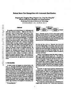
Abstract This paper presents a novel approach to utilizing high level knowledge for the problem of scene recognition in an active vision framework, which we call active scene recognition. In traditional approaches, high level knowledge is used in the post-processing to combine the outputs of the object detectors to achieve better classification performance. In contrast, the proposed approach employs high level knowledge actively by implementing an interaction between a reasoning module and a sensory module (Figure 1). Following this paradigm, we implemented an active scene recognizer and evaluated it with a dataset of 20 scenes and 100+ objects. We also extended it to the analysis of dynamic scenes for activity recognition with attributes. Experiments demonstrate the effectiveness of the active paradigm in introducing attention and additional constraints into the sensing process.

Figure 1. Overview of the active approach for scene recognition.

In this paper we propose a new approach to scene understanding in the paradigm of active vision. Central to the approach is a bio-inspired attention mechanism. Human perception is active and exploratory. We continuously shift our gaze to different locations in the scene. After recognizing objects, we will fixate again at a new location, and so on. Humans interpret visual input by using their knowledge of actions and objects, along with the language used for representing this information. It is clear that when we analyze a complex scene, visual processes continuously interact with our high-level knowledge, some of which is represented in the form of language. In some sense, perception and language are engaged in an interaction, as they exchange information that leads to meaning and understanding. This idea is applied to the simplest interpretation problem, scene recognition, in this paper. The proposed system consists of two modules: (1) the reasoning module, which obtains higher level knowledge about scene and object relations, proposes attentional instructions to the sensory module and draws conclusions about the contents of the scene; (2) the sensory module, which includes a set of visual operators responsible for extracting features from images, detecting and localizing objects and actions. The novelty of the proposed active paradigm is that the sensory module does

1. Introduction The paradigm of Active Vision [1, 2, 3, 18] had invigorated Computer Vision research in the early 1990s. The ideas were inspired by the observation that in nature vision is used by systems that are active and purposive. By studying visual perception in isolation, we often end up with more complicated formulations and under-constrained problems. Thus, the Active Vision paradigm proposed that visual perception should be studied as a dynamic and purposive process for active observers that can control their imaging mechanism. Most previous work in this paradigm was concerned with low level robot vision problems, and applied the ideas to shape reconstruction and navigational problems, such as motion estimation, obstacle avoidance, surveillance and path planning. Higher level tasks of scene understanding and recognition have not been sufficiently studied in this framework. These problems require combining high level knowledge and reasoning procedures with low-level image processing and a systematic mechanism for doing so. 1

not passively process the image; instead, it is guided by the reasoning module, which decides what and where the sensory module should process next. Thus the sensory module shifts the focus of attention to a small number of objects at selected locations of the scene. This leads to faster and more accurate scene recognition. Another novelty in the proposed approach is that the reasoning module can automatically obtain high-level knowledge from textual corpus. Thus the proposed approach can recognize scenes that it has never seen before. Figure 1 illustrates the interaction between the two modules, which is modeled as an iterative process. Within each iteration, the reasoning module decides on what and where to detect next and expects the sensory module to reply with some results after applying the visual operators. The reasoning module thus provides a focus of attention for the sensory module, which can be an object to be detected and a place to be examined. For the problem of scene recognition, the interaction between the two modules is simple. (See Figure 6 for examples of the interaction over a given image.) However, our framework is more general. In Section 5 we discuss the extension of the framework to dynamic scene understanding. In this case the goal is to interpret the activity in the video. An activity is described by a set of quantities: the human, the tools, the objects, the motion, and the scene involved in the activity. Each of the quantities has many possible instances which can be described by their attributes (e.g., adjectives of nouns and adverbs of verbs). Thus the reasoning module at every iteration has to decide which quantity and which attribute to compute next. This procedure can be implemented in a hierarchical model of the proposed active scheme. The rest of the paper is organized as follows: in the next section, we review related work; Section 3 describes an implementation of the proposed paradigm; in Section 4 we experimentally evaluate the active scene recognizer; in Section 5 we discuss how our framework can be generalized to object recognition and dynamic scene interpretation, and we demonstrate the ideas on the problem of recognizing hand activities on a small dataset; finally we draw conclusions in Section 6.

2. Related Works Recognition by Components: The methodology for object, scene and activity recognition in this paper follows the idea of “recognition by components”, which can be traced back to early work by Biederman [4]. In this methodology, scenes are recognized by detecting the inside objects [14], objects are recognized by detecting their parts or attributes [12], and activities are recognized by detecting the motions, objects and contexts involved in the activities [11]. However, all previous works employ passive approaches. As a result, they need to run through all object/attribute de-

tectors over the testing images and videos before making the final conclusion. In this paper we explore an active approach, which aims at greatly reducing the number of object/attribute detectors needed for recognition of objects, scenes and activities. Active Learning and Active Testing: Our work is a type of active testing and is closely related to the visual “20 question” game described in [5]. While the approach in [5] needs human annotators to answer the questions posed by the computer, our approach is fully automated without a human in the loop. To select the optimal objects/attributes, we use the criterion of Maximum Information Gain, which have been widely used for active learning of objects and scenes [21, 25]. Information theory also have been used for object localization in application of face detection [22]. Employing Ontological Knowledge in Computer Vision System for Scene Interpretation: Ontological knowledge plays an important role in the reasoning and learning system of human. For example, in the problem of scene recognition, if we know that coast is a type of outdoor scene and also know that it is unlikely to find bookshelves therein. Hence, we do not need to apply the bookshelves detectors in the possible coast scene image. The work in [23] takes advantage of this type of knowledge in object detection. Similarly, the knowledge about objects and attributes is employed in [12]. Extending the knowledge about object hierarchy is employed in [16]. In this paper, we further explore the ontological knowledge about activities and attributes and present a pilot study using a hand activity dataset.

3. The Approach 3.1. System Overview The proposed active scene recognizer classifies a scene by iteratively detecting the objects inside it. In the k-th iteration, the reasoning module provides an attentional instruction to the sensory module to search for an object Ok within a particular region Lk in the image. Then the sensory module runs the corresponding object detector and returns a response, which is the highest detection score dk and the object’s location lk . The reasoning module receives this response, analyses it and starts a new iteration. This iteration continues until some terminating criteria are satisfied. To implement such an active scene recognizer, we need to solve the the following problems: (1) sensory modules for object detection; (2) a reasoning module for predicting the scene class based on the sensory module’s responses; (3) a strategy for deciding which object and where in the scene the sensory module should process in the next iteration; and (4) a strategy for initializing and terminating the iteration. We will describe these components in the rest of this sec-

tion.

3.2. Scene Recognition by Object Detection In the proposed framework, the reasoning module decides the scene class S based on the responses X from the sensory module, which we call Scene Recognition by Object Detection (SROD). The optimal scene class of the given image belongs to the one that maximizes the probability: S ∗ = arg max p(S|X),

(1)

S∈[1:M ]

where M is the number of scene classes. The responses from the sensory module are a detection score and a detection bounding box. We only consider the objects’ vertical positions, since they are more consistent within the images of the same scene class [23]. An object’s vertical position is represented by a profile of the mask formed by the object’s bounding box (see Figure 2 for an example). The object’s mask formed by the object’s bounding box is normalized to 256 × 256 pixels, and the profile is the histogram of pixels within the object’s mask along the vertical direction. By this compact representation, we not only record the object’s vertical location, but also record the object’s scales along the horizontal and vertical direction. In the following, we denote this representation of an object’s location as lk . As described above, in each iteration, the sensory module returns a detection score di and detected location li for the expected object Oi . Thus at step k, we have accumulated a list of detected score d1:k and corresponding locations l1:k . Given X = (d1:k , l1:k ), the probability of a scene S is : P (S|X) = p(S|d1:k , l1:k ) ∝ p(d1:k , l1:k |S) = p(d1:k |S)p(l1:k |S).

(2)

In the above equation, we assume d1:k and l1:k are independent given S. We approximate p(d1:k |S) by the inner product of d1:k and d˜S1:k , where d˜S1:k is the mean d1:k of training examples for scene class S. Similarly, p(l1:k |S) is approxiS mated by the inner product of l1:k and ˜l1:k . The advantage of this approximation is its simplicity and flexibility. We need to update the list of selected object in each iteration. If we adopt a parametric model for p(d1:k |S) and p(l1:k |S), we would need to learn the parameters for all permutations of O1:k , k = 1, ..., N , where N is the total number of object categories in the dataset. For large N 1 , such scheme would not work simply because of the computational constraints. Using a parameter-free approach, we avoid this difficulty. 1 In

our dataset, N > 100

(a)

(b)

(c)

Figure 2. Representation of the object’s location: (a) an object’s bounding box; (b) the binary mask formed by the bounding box; (a) the profile of the object’s binary mask along the vertical direction.

3.3. Detecting Objects by The Sensory Module The task of the sensory module is to detect the object required by the reasoning module and return a response. In this paper, we applied three object detectors: a Spatial Pyramid Matching object detector [13], a latent SVM object detector [8] and the texture classifier by Hoime [10]. For each object class, we train all three object detectors and then select the one with the highest detection accuracy on a validation dataset to use in the test. Given a test image, the object detector will find a few candidates with corresponding detection scores. The one with the highest score is selected and sent to the reasoning module. The detection scores are normalized by Platt scaling [19] to obtain probabilistic estimates.

3.4. Attentional Instructions by The Reasoning Module The interaction between the reasoning and sensory module at iteration k starts from an attentional instruction issued by the reasoning module, based on its observation history. In this paper, the attentional instruction in iteration k includes what to look for, i.e., the object to detect (denoted as Ok ) and where to look, i.e., the regions to detect (denoted as Lk ). The criterion to select Ok and Lk is to maximize the expected information gain about the scene in the test image due to the response of this object detector: {Ok∗ , L∗k } = arg max I(S; dk , lk |d1:k−1 , l1:k−1 ),

(3)

˜k−1 , Ok ∈N Lk ∈Lk

˜k−1 denotes the set of indices of objects that have where N not been detected until iteration k, Lk denotes the search space of Ok ’s location. The global optimization procedure is approximated by two local optimization procedures. In the first step, we select Ok based on the maximum expected information gain criterion: Ok∗ = arg max I(S; dk , lk |d1:k−1 , l1:k−1 ).

(4)

˜k−1 Ok ∈N

S Then L∗k is selected by thresholding ˜lOk∗ = ES [˜lO ∗ ], the k ∗ expected location of object Ok across all scene classes.

The expected information gain of Ok given the previous response d1:k−1 and l1:k−1 is defined as: I(S;dk , lk |d1:k−1 , l1:k−1 ) X = p(dk , lk |d1:k−1 , l1:k−1 ) dk ∈D,lk ∈Lk

× KL[p(S|d1:k , l1:k ), p(S|d1:k−1 , l1:k−1 )].

(5)

The KL divergence on the right side of Equation 5 can easily be computed after applying Equation 2. To compute the first term on the right side of Equation 5, we factorize it as follows: p(dk , lk |d1:k−1 , l1:k−1 ) = p(dk |d1:k−1 , l1:k−1 )p(lk |d1:k , l1:k−1 ).

(6)

The two terms on the right side of the above equation can be efficiently computed by their conditional probability with respect to S p(dk |d1:k−1 , l1:k−1 ) =

M X

M X

p(dk |S, d1:k−1 , l1:k−1 )p(S|d1:k−1 , l1:k−1 ) p(dk |S)p(S|d1:k−1 , l1:k−1 ),

(7)

S=1

where we assume dk is independent of d1:k−1 and l1:k−1 given S. p(dk |S) can be computed by introducing the binary variable ek , which indicates whether object Ok appears in the scene or not: X p(dk |S) = p(dk |ek , S)p(ek |S) (8) ek ∈{0,1}

=

X

p(dk |ek )p(ek |S).

yk ∼N (µyk , σy2k ),

(10)

hk ∼N (µhk , σh2 k ),

(11)

2 wk ∼N (µwk , σw ). k

(12)

The means and variances of these Gaussian distributions are estimated from the training set. Thus the problem of drawing a sample of lk becomes the problem of drawing a sample of yk , hk , wk from three Gaussian distributions. After drawing samples of dk and lk , we substitute them into Equation 5 to compute the expected information gain for Ok . Then among all possible Ok ’s, we select the object that yields the maximum expected information gain, Ok∗ . Finally, L∗k is S selected by thresholding ES [˜lO ∗ ]. k

3.5. Initializing and Terminating the Iteration The interaction between two modules starts from the first object and its expected location, which are provided by the reasoning module. We select the object O1 that maximizes the mutual information

S=1

=

and we draw samples of dk uniformly. Lk can be parameterized by three parameters: the center position of Ok , yk ; the horizontal extent of Ok , wk ; and the vertical extent of Ok , hk . We model these parameters by Gaussian distributions

(9)

ek ∈{0,1}

p(ek |S) encodes the high-level knowledge about the relationship between scene S and object Ok . One way to obtain it is to count the object labels in the training image set. Otherwise, we can obtain it from textual corpus. In Section 3.6, we will describe an approach to do so. p(dk |ek ) encodes the information about the accuracy of different object detectors. It can be computed from the training set as a posterior of a multinomial distribution with a Dirichlet prior Dir(α), where α represents the number of prior observations of dk given a particular ek . Through all experiments in this paper, we set the parameter α = 1. p(lk |d1:k , l1:k−1 ) can be computed in a similar fashion. Finally, we note that the expectation in Equation (5) needs to be computed at a set of sampling points of dk (denoted as D) and a set of sampling points of lk (denoted as Lk ). D is within a one dimensional space between 0 and 1

O1∗ = arg max I(S; d1 , l1 ).

(13)

O1 ∈[1:N ]

To terminate the iteration, we can either stop after a fixed number of iterations (e.g., the 20 question game), or stop when the expected information gain at each iteration is below a threshold. In our experiments, we found that 30 iterations are sufficient to produce competitive recognition results.

3.6. Obtaining Knowledge By Language Tools The proposed approach requires high-level knowledge describing the relationship between scene and object, P (ek |S). This knowledge can be obtained from textual corpus in an automatic manner. From the generic text obtained from the English Gigaword corpus [9], we count the number of times when scene S co-occurs with object Ok , #(S, Ok ) and the number of times when scene S occurs in Gigaword, #(S). Then we define P (ek |S) as P (ek |S) =

#(S, Ok ) . #(S)

(14)

In order to ensure that P (ek |S) captures the correct sense of the words, we use WordNet to determine the synonyms and hyponymns of the name of scenes and objects, and add them in the counting. In this scenario, no spatial information will be used in the active scene recognition model (Equations 1 through 2), and the reasoning module will only predict the object to be searched in the next iteration (Equations 3 through 13).

Figure 3. Comparison of classification performance of different approaches (GIST+SVM vs. BoW+SVM vs. CART vs. SROD). We also illustrate the “ideal” performance of CART and SROD, where we use the object ground truths as the outputs of object detectors. They are represented as “(CART)” and “(SROD)” in the figure respectively.

4. Experiments 4.1. Image Datasets We evaluate the proposed approach using a subset of the SUN image set from [7]. There is a total of 20 scenes and 127 objects in our image set. For each scene, we select 30 images for training and 20 images for testing. The object detectors are trained using a dataset that is separated from the training/testing scene images as described in [7].

4.2. Performance of the Scene Recognizer In the first experiment, we evaluate the scene recognizer (SROD) as described in Equation 2 while all objects are detected. The “ideal” SROD, where we use the object ground truths as the outputs of object detectors, is also evaluated to illustrate the upper limit of the performance of SROD. Three baseline algorithms are evaluated as listed below: • SVM using GIST [17] features • SVM using Bag-of-Words (BoW), where two types of local features are used, SIFT [15] and opponent SIFT [24], and 500 visual words are used for each of them • Classification and Regression Tree (CART) [6] using the object detection scores as features. The “ideal” CART, where the object ground truth is used as features, is also evaluated to illustrate the upper limit of the performance of CART. Figure 3 compares the performance of these baseline algorithms and the SROD approach. The SROD approach significantly outperforms all the baseline algorithms. This result confirms the effectiveness of object-based approaches in interpreting complex scenes and the robustness of the SROD approach to the errors in object detection. It is worth to emphasize that there is still a lot of room to improve the current object-based scene recognizer, as suggested by the performance of the ideal SROD.

Figure 4. Classification performance of different approaches (GIST+SVM vs. BoW+SVM vs. CART vs. SROD) with respect to the number of training images.

In addition, we evaluate the robustness of these scene recognition approaches with respect to the size of training samples. We randomly select a number of training examples from the training image set for each scene class and repeat the experiments three times. The mean and standard deviation of the average accuracy when using 5, 10, 15, 20, 25 and 30 training examples are reported in Figure 4. The proposed SROD method achieves substantially better performance than all baseline algorithms, including the CART algorithm that uses the same outputs of object detectors. Finally, we evaluate the performance of the SROD approach when high-level knowledge is obtained from textual corpus only, which is marked with a red arrow in Figure 4. With ZERO training examples, we achieve 37% accuracy, much higher than the chance level of 5%. This is equivalent to having 5 training examples in classifiers using GIST and BoW features. This result again highlights the advantage of the object-based scene classifier.

4.3. Comparison of the Active Scene Recognizer vs. the Passive Scene Recognizer In this experiment, we compare the proposed active scene recognizer with two baseline algorithms and the results are presented in Figure 5. Both baseline uses the same SROD formulation but employ different strategies to select the object in each iteration. The first baseline (denoted as “DT” in Figure 5) follows a fixed object order, which is provided by the CART algorithm, and the second baseline (denoted as “Rand” in Figure 5) just randomly selects an object from the remaining object pool. Object selection obviously has a big impact on the performance of scene recognition, since both the proposed active approach and the “DT” approach significantly outperform the “Rand” approach. The result also shows that the active approach is superior to the “DT” approach that is passive: the active approach can achieve competitive performance after selecting 30 objects while the passive “DT” approach needs 60 ob-

Figure 7. Hierarchical active scheme for dynamic scene recognition, where each iteration invokes four steps: (1) attentional instruction from the activity-level reasoning module; (2) attentional instruction from the quantity-level reasoning module; (3) responses from attribute detectors; (4) responses from the quantitylevel reasoning module. Quantity Figure 5. Classification performance of different object selection strategies (active vs. passive vs. random) in the object-based scene recognizer with respect to the number of object detectors.

jects. Furthermore, the object’s expected location provided by the reasoning module in the active approach not only reduces the spatial search space to be about 1/3 to 1/2 of the whole image but also reduces the false positives in the sensory module’s response. As a result, the active approach achieves 3% to 4% performance gain compared to the passive approach.

4.4. Visualization of the Interaction between the Sensory Module and the Reasoning Module Figure 6 illustrates a few iterations of the active scene recognizer performed on a test image. It shows that after detecting twenty objects, the reasoning module is able to decide the correct scene class with high confidence.

5. Dynamic Scene Recognition There are two key premises in the proposed active scheme: (1) a quantity can be recognized by accumulating evidences from its components; (2) the components can be assumed to be independent given the quantity. Given these two premises, the active scheme can be applied to select a small number of components to recognize the quantity without impairing the performance. In the previous section, we have applied this active scheme to recognize static scenes. However, this active scheme can also be applied to recognize objects by their parts and activities by their motion and object properties. In this section, we will demonstrate the application of the active scheme in activity recognition. A big challenge in this problem is that the components are heterogeneous. While static scenes only involve a single quantity, i.e., objects, activities are described by different quantities, including motion, objects and tools, scenes, temporal properties, etc. To alleviate this problem, we propose a hierarchical active scheme for dynamic scene recognition. Figure 7 presents this method. In this scheme, each iteration in-

Tools

Motion

Attribute Color Texture Elongation Convexity Frequency Motion variation Motion spectrum Duration

e=1 silver bristle yes yes high large sparse long

e=0 other colors non-bristle no no low small non-sparse short

Table 1. Activity attributes in the hand activity dataset.

vokes four steps: (1) using the maximum information gain criterion, the activity-level reasoning module sends an attentional instruction to the quantity-level reasoning module that indicates the desired quantity (e.g., motion or objects); (2) the quantity-level reasoning module then sends an attentional instruction to the sensory module that indicates the desired attributes (e.g., object color/texture, motion properties); (3) the sensory module applies the corresponding detectors and returns the detector’s response to the the quantity-level reasoning module; (4) finally, the quantity-level reasoning module returns the likelihood of the desired quantity to the activity-level reasoning module. To demonstrate this idea, we used 30 short video sequences of 5 hand actions from a dataset collected from the commercially available PBS Sprouts craft show for kids (the hand activity data set). The activities are coloring, drawing, cutting, painting, and gluing. 20 sequences were used for training and the rest for testing. Two quantities are considered in recognizing an activity: the characteristics of tools and the characteristics of motion. Four attributes are defined for the characteristics of tools, including color, texture, elongation, and convexity; and four attributes are defined for the characteristics of motion, including frequency, motion variation, motion spectrum, and duration. The details of these quantities and attributes are described in Table 1. The sensory module includes detectors for the 8 attributes of tools/motion. To detect these attributes, we need to segment the hand and tools from the videos. Figure 8 illustrates these procedures, which are described as follows: 1. Hand regions Sh are segmented by applying a variant

Expected Object Ok :

O1 wall

O2 person

Expected Location Lk :

Sensory Module’s Response (dk , lk ):

Reasoning module’s Belief P (S|d1:k , l1:k ) and S ∗

O3 books

... ...

O10 sink

... ...

O20 toilet

... ...

...

...

...

...

...

...

...

...

...

Figure 6. Visualization of the iterations between the reasoning module and the sensory module in an active scene recognition process. The detected regions with detection score greater than 0.5 are highlighted with a red bounding box.

of the color segmentation approach based on Conditional Random Fields (CRF) [20] using a trained skin color model. 2. Moving regions of hands and tools, Sf , are segmented by applying another CRF over the optical flow fields. 3. Applying a binary XOR operation on the two regions and produce a segmentation of tools, ST . 4. Fitting a minimum volume ellipse over the edge map of ST , and provide the tool region. Figure 9 shows the estimated ellipse enclosing the detected tool over some sample image frames from the dataset. This ellipse, together with ST , is then used as a mask to detect object-related attributes. The color and texture attributes were computed from histograms of color and wavelet-filter outputs, and the shape attributes were derived from region properties of the convex hull of the object and the fitted ellipse. The motion attributes were computed from the spectrum of the average optical flow over the sequence and the variation of the flow. Table 2 shows the interactions between the reasoning modules and the sensory modules for one of the testing videos. Here the sensory module only needed to detect two attributes before the reasoning module arrived at the correct conclusion. Overall, 8 out of 10 testing videos were recognized correctly after detecting two to three attributes, while the remaining two testing videos could not be recognized

Figure 8. Procedures to extract hands and tools from the hand activity video sequence. (1) inputs hand and flow segmentation from the test image. (2) applies a threshold tf to remove regions with flow that are different from the hand region to obtain mask of tools in (3). (4) performs edge detection and (5) fits the best ellipse over the edge fragments to locate the tool.

Figure 9. Sample frames for 10 testing videos in the hand action dataset. Frames in the same column belong to the same activity class: (from left to right) coloring, cutting, drawing, gluing, painting. The detected tool is fit with an ellipse.

correctly even after detecting all the attributes. This is because of errors in the segmentation, the choice of attributes

Iteration Expected quantity Expected attribute Sensory module’s response Reasoning module’s conclusion Reasoning module’s confidence

1 Tools

2 Tools

3 Tools

4 Motion

Elongation Color

Texture

Duration

0.770

1.000

0.656

0.813

Coloring

Painting

Painting

Painting

0.257

0.770

0.865

0.838

Table 2. An example of interactions between the reasoning module and the sensory module for hand activity recognition, where the ground truth of the activity class is painting.

and the small set of training samples.

6. Conclusion and Future Work We proposed a new framework for scene recognition within the active vision paradigm. In our framework, the sensory module is guided by attentional instructions from the reasoning module and employs detectors of a small set of objects within selected regions. The attention mechanism is realized using an information theoretic approach, with the idea that every detected object should maximize the added information for scene recognition. Our framework is evaluated in a static scene dataset and shows the advantage over the passive approach. Also we discussed how it can be generalized to object recognition and dynamic scene analysis, and gave a proof of concept by implementing it for attribute based activity recognition. In the current implementation, we have assumed that objects are independent given the scene class. Though this assumption simplifies the formulation, this is not necessarily true in general. In the future, we plan to remove this assumption and design a scene recognition model that better represents the complex scenes in the real world. Also, we will perform a comprehensive study of the proposed approach using larger image/video datasets to investigate the impact of the active paradigm.

References [1] J. Aloimonos, I. Weiss, and A. Bandopadhay. Active Vision. IJCV, 2:333–356, 1988. 1 [2] R. Bajcsy. Active Perception. Proceedings of the IEEE, 76:996–1005, 1988. 1 [3] D. H. Ballard. Animate Vision. Artificial Intelligence, 48:57–86, 1991. 1 [4] I. Biederman. Recognition-by-Components: A Theory of Human Image Understanding. Psychological Review, 94:115–147, 1987. 2

[5] S. Branson, C. Wah, B. Babenko, F. Schroff, P. Welinder, P. Perona, and S. Belongie. Visual Recognition with Humans in the Loop. In ECCV, 2010. 2 [6] L. Breiman, J. Friedman, C. J. Stone, and R. Olshen. Classification and Regression Trees. Chapman and Hall/CRC, 1984. 5 [7] M. J. Choi, J. Lim, A. Torralba, and A. S. Willsky. Exploiting Hierarchical Context on a Large Database of Object Categories. In CVPR, 2010. 5 [8] P. Felzenszwalb, R. Girshick, D. McAllester, and D. Ramanan. Object Detection with Discriminatively Trained Part Based Models. PAMI, 32(9):1627 – 1645, 2010. 3 [9] D. Graff. English Gigaword. In Linguistic Data Consortium, 2003. 4 [10] D. Hoiem, A. Efros, and M. Hebert. Automatic Photo Popup. In ACM SIGGRAPH, 2005. 3 [11] N. Ikizler-Cinbis and S. Sclaroff. Object, Scene and Actions: Combining Multiple Features for Human Action Recognition. In ECCV, 2010. 2 [12] H. N. Lampert, C. H. and S. Harmeling. Learning To Detect Unseen Object Classes by Between-Class Attribute Transfer. In CVPR, 2009. 2 [13] S. Lazebnik, C. Schmid, and J. Ponce. Beyond Bags of Features: Spatial Pyramid Matching for Recognizing Natural Scene Categories. In CVPR, 2006. 3 [14] L.-J. Li, H. Su, E. P. Xing, and L. Fei-Fei. Object Bank: A High-Level Image Representation for Scene Classification & Semantic Feature Sparsification. In NIPS, 2010. 2 [15] D. G. Lowe. Distinctive Image Features from Scale-invariant Keypoints. IJCV, 20:91–110, 2004. 5 [16] M. Marszalek and C. Schmid. Semantic Hierarchies for Visual Object Recognition. In CVPR, 2007. 2 [17] A. Oliva and A. Torralba. Modeling the Shape of the Scene: a Holistic Representation of the Spatial Envelope. IJCV, 42:145–175, 2001. 5 [18] J. olof Eklundh, P. Nordlund, and T. Uhlin. Issues in Active Vision: Attention and Cue Integration/Selection. In BMVC, pages 1–12, 1996. 1 [19] J. C. Platt. Probabilities for SV Machines. In Advances in Large Margin Classifiers, 1999. 3 [20] C. Rother, V. Kolmogorov, and A. Blake. GrabCut: interactive Foreground Extraction using Iterated Graph Cuts. ACM Trans. Graph., 23(3):309–314, 2004. 7 [21] B. Siddiquie and A. Gupta. Beyond Active Noun Tagging: Modeling Contextual Interactions for Multi-Class Active Learning. In CVPR, 2010. 2 [22] R. Sznitman and B. Jedynak. Active Testing for Face Detection and Localization. PAMI, 2010. 2 [23] A. Torralba. Contextual Priming for Object Detection. IJCV, 53(2):153–167, 2003. 2, 3 [24] van de Sande, K. E. A., T. Gevers, and C. G. M. Snoek. Evaluating Color Descriptors for Object and Scene Recognition. PAMI, 32(9):1582–1596, 2010. 5 [25] S. Vijayanarasimhan and K. Grauman. Cost-Sensitive Active Visual Category Learning. IJCV, 2010. 2