Scene Text Recognition using Higher Order Language Priors

Mishra et al.: Scene Text Recognition using Higher Order Language Priors

1

Scene Text Recognition using Higher Order Language Priors Anand Mishra1

1

CVIT IIIT Hyderabad Hyderabad, India

2

INRIA - WILLOW ENS Paris, France

http://researchweb.iiit.ac.in/~anand.mishra/

Karteek Alahari2 http://www.di.ens.fr/~alahari/

C.V. Jawahar

1

http://www.iiit.ac.in/~jawahar/

Abstract The problem of recognizing text in images taken in the wild has gained significant attention from the computer vision community in recent years. Contrary to recognition of printed documents, recognizing scene text is a challenging problem. We focus on the problem of recognizing text extracted from natural scene images and the web. Significant attempts have been made to address this problem in the recent past. However, many of these works benefit from the availability of strong context, which naturally limits their applicability. In this work we present a framework that uses a higher order prior computed from an English dictionary to recognize a word, which may or may not be a part of the dictionary. We show experimental results on publicly available datasets. Furthermore, we introduce a large challenging word dataset with five thousand words to evaluate various steps of our method exhaustively. The main contributions of this work are: (1) We present a framework, which incorporates higher order statistical language models to recognize words in an unconstrained manner (i.e. we overcome the need for restricted word lists, and instead use an English dictionary to compute the priors). (2) We achieve significant improvement (more than 20%) in word recognition accuracies without using a restricted word list. (3) We introduce a large word recognition dataset (atleast 5 times larger than other public datasets) with character level annotation and benchmark it.

1 Introduction On one extreme Optical Character Recognition (OCR) is considered as one of the most successful applications of computer vision, and on the other hand text images taken from street scenes, video sequences, text-captcha, and born-digital (the web and email) images are extremely challenging to recognize. The computer vision community has shown a huge interest in this problem of text understanding in recent years. It involves various sub-problems such as text detection, isolated character recognition, word recognition. These sub-problems are either looked at individually [3, 6, 8] or jointly [14, 21]. Thanks to the recent work of [6, 8], text detection accuracies have significantly improved, but they were less successful in recognizing words. Recent works on word recognition [13, 20, 21] have addressed this to some extent, but in a limited setting where a list of words is provided for each image (referred to as c 2012. The copyright of this document resides with its authors.

It may be distributed unchanged freely in print or electronic forms.

2

Mishra et al.: Scene Text Recognition using Higher Order Language Priors

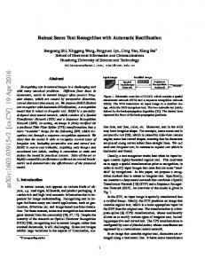
Figure 1: Some sample images from the IIIT 5K-word dataset. Images in this dataset contain examples that have a large variety of appearances, and are much more complex than the ones seen in typical OCR datasets. a small size lexicon). Such strong assumptions, although effective, are valid only for limited applications, e.g. recognizing a certain text in a grocery store, where a list of grocery items can serve as a lexicon. However, the availability of such lists is not always possible, or the word may not be part of the given list. In other words, text recognition performance in a general setting leaves a lot to be desired. In this paper we rely on a large English dictionary (with around 0.5 million words, provided by authors of [23]) instead of an image specific word list. We present a framework that uses the n-gram information in the language to address the problem of small size lexicons. The use of n-grams as a post-processor is not new to the OCR community [18]. We combine these useful priors into a higher order potential function in a Conditional Random Field (CRF) [11] model defined on the image. The use of higher order potentials not only deals with weak character detections but also allows us to recognize non-dictionary words, as shown in the latter sections. Another issue with many of the previously published works [13, 17, 21] is that they were evaluated on datasets containing a few hundred words. For a comprehensive evaluation of methods, we need a large dataset with diversity. Thus, we introduce a dataset with 5000 word images referred to as the IIIT 5K-word dataset. The dataset contains words from both street scene texts and born-digital images. Note that automatically extracting text from born-digital images has many applications such as improved indexing and retrieval of web content, enhanced content accessibility, content filtering, e.g. advertisements or spam emails. Moreover, the IIIT 5K-word dataset will also be useful to evaluate the performance of character detection module, as we also provide character bounding box level annotation for this dataset. The main contributions of this work can be summarized as: (1) We relax the assumption of recognizing a word with the help of small size lexicons, unlike previously published work on this problem [13, 20, 21]. (2) We present a CRF framework, which incorporates higher order statistical language models to infer the word (Section 2). It allows us to by-pass the use of edit distance based measures.1 (3) We introduce a large dataset of scene text and borndigital images harvested from Google image search. We have evaluated and benchmarked this dataset (Section 3). Our method achieves a significant improvement of over 20% on the IIIT 5K-word and other datasets.

2 The Recognition Model We propose a CRF based model for recognizing words. The CRF is defined over a set of random variables x = {xi |i ∈ V }, where V = {1, 2, ..., n}. Each random variable xi denotes a potential character in the word, and can take a label from the label set L = {l1 , l2 , ..., lk } ∪ ε , which is the set of English characters and digits, and a null label to suppress weak detections 1 The edit distance between two strings is defined as the minimum number of edits needed to transform one string into the other. For example words ‘BMVC’ and ‘BMVA’ have edit distance of one. A single edit distance computation has time complexity of O(|s1 ||s2 |) where s1 and s2 are the length of the string. Moreover, the edit distance based measure can not be used for the problem we consider, i.e. out-of-vocabulary recognition.

Mishra et al.: Scene Text Recognition using Higher Order Language Priors

3

(similar to [13]). The most likely word represented by the set of characters xi is found by minimizing the energy function, E : Ln → R, corresponding to the random field. The energy function E(·) can be typically written as sum of potential functions: E(x) =

∑ ψc (xc ),

(1)

c∈C

where C represents a set of subsets of V , i.e. cliques. Here xc is the set of random variables included in a clique c. The set of potential characters is obtained by the character detection step discussed in Section 2.1. The neighbourhood relations among characters, which determine the structure of the random field, are based on the spatial arrangement of characters in the word image. Details of the potentials defined on these relations are given in Section 2.2.

2.1 Detecting Characters The first step in our approach is to detect potential locations of characters in a word image. We apply a sliding window based approach to achieve this. Sliding window based detectors have been very successful for challenging tasks, such as face [19] and pedestrian [7] detection. Although character detection is similar to such problems, it has its unique challenges. Firstly, there is the issue of dealing with a large number of categories (62 in all). Secondly, often, parts of a character or a part of two consecutive characters are similar in appearance to another character. We use a standard sliding window based approach with character aspect ratio prior, similar to [13]. This approach produces many potential character windows, but not all of them are useful for recognizing words. Dealing with large number of false positives becomes challenging, especially because we use a dictionary to learn the context. Moreover, our objective is to recognize a word that may not be in the given dictionary. In Section 3 we study the trade-off between true and false positives, and its effect on the overall word recognition accuracy. We exhaustively evaluate the performance of character detection on IIIT 5K-word dataset with various ways of pruning weak detections.

2.2 Recognizing Words The character detection step provides us with a large set of windows potentially containing characters within them. Our goal is to infer the most likely word from this set of characters. We formulate this problem as that of minimizing the energy in (1), where the best energy solution represents the ground truth word we aim to find. The energy function defined over cliques of size one is referred to as a unary potential, and that of size two is referred to as a pairwise potential. The potentials defined over cliques of size greater than two are commonly known as higher order potentials. For introducing higher order, we add an auxiliary variable xac for every clique c ∈ C. This auxiliary variable takes label from a label set Le . In our case the extended label set Le contains all possible h-gram combination present in the lexicons plus one, assuming we model CRF of order h. We define a very high cost for an auxiliary variable to take a label which is not present in the dictionary. Increasing the order of the CRF allows us to capture a larger context. However, arbitrarily increasing order may force a recognized word to be a dictionary word. Since, we also aim to recognize words which may not be in a dictionary, we need to be mindful in choosing the order of the CRF. This is investigated in Section 3. 2.2.1 Graph Construction and Energy Formulation We solve the energy minimization problem on a corresponding graph, where each random variable is represented as a node in the graph. We begin by ordering the character

4

Mishra et al.: Scene Text Recognition using Higher Order Language Priors

(a)

(b)

Figure 2: The proposed graphical model. (a) Each (non-auxiliary) node takes one of the labels from the label set {l1 , l2 , ..., lk } ∪ ε , where li represents an English character or a digit, and ε is a null label. The auxiliary nodes can take labels from the set of all h-grams that are present in an English dictionary, and an additional label to enforce high cost for a h-gram that is not present in the dictionary. Labels {L1 , L2 , ..., Ln } are the possible trigrams in the dictionary whereas label Ln+1 represents trigrams that never occur in the dictionary. (b) An example word image with the proposed model: Tri-grams like OPE, PEN have very high frequency in an English dictionary (> 1500), and thus are of low cost. Integrating higher order information into the CRF results in the correct word. windows based on their horizontal location, and add one node each for every window sequentially from left to right. The nodes are then connected by edges. To enforce higher order constraints, we add an auxiliary node for every clique of size h, where h is the order of the CRF. Each (non-auxiliary) node in this graph takes one label from the label set L = {l1 , l2 , ..., lk } ∪ ε . Note that each li is an English character or digit. The cost associated with such labeling is known as unary cost. Further, there is also a cost associated with two neighboring nodes taking some label li and l j respectively, which is known as pairwise cost. This cost is learnt from the dictionary. The auxiliary nodes in the graph take labels from the extended label set Le . Each element of Le represents one of the h-grams present in the dictionary and an additional label to assign constant (high) cost to all those h-grams that are not present in the dictionary. The proposed graphical model is shown and explained in Figure 2. We show a CRF of order three for clarity, but it can be extended to any order without loss of generality. Unary Cost. The unary cost of a node taking a character label is determined by the SVM confidence. The unary term ψ1 , which denotes the cost of a node xi taking label l j , is defined as: ψ1 (xi = l j ) = 1 − p(l j |xi ), (2) where p(l j |xi ) is the SVM score of character class l j for node xi . Pairwise Cost. The pairwise cost of two neighboring nodes xi and x j taking a pair of character labels li and l j respectively is determined by their probability of occurrence in the dictionary as: ψ2 (xi , x j ) = λl (1 − p(li, l j )), (3) where p(li , l j ) is the joint probability of the character pair li and l j occurring together in the dictionary. The parameter λl determines the penalty for a character pair occurring in the lexicon.

Mishra et al.: Scene Text Recognition using Higher Order Language Priors

5

Higher Order Cost. The higher order costs in the CRF energy are decomposed into unary and pairwise costs, similar to the approach described in [16]. For simplicity, let us assume we use a CRF order h = 3. Then, an auxiliary node corresponding to every clique of size 3 is added to the graph, and every auxiliary node takes one of the labels from the extended label set Le = {L1 , L2 , ...Ln } ∪ Ln+1 , where labels L1 . . . Ln represent all possible trigrams in the dictionary. The additional label Ln+1 denotes all those trigrams that do not occur in the dictionary. The unary cost for the auxiliary variable is defined as:  0 if i ∈ {1,2, ..., n}, (4) ψ1a (xi = Li ) = λa otherwise, where λa is a constant and penalizes all those character triples which are not in the dictionary. The pairwise cost between an auxiliary node xi taking a label Lk = li l j lk and left-most non-auxiliary node in the clique, x j , taking a label ll is given by:

ψ2a (xi

= Lk , x j = ll ) =



0 λ a′

if l = i otherwise,

(5)

where λa′ penalizes a disagreement between the auxiliary and non-auxiliary nodes. Inference. After computing the unary, pairwise and higher order terms, we use the sequential tree-reweighted message passing (TRW- S) algorithm [10] to minimize the energy function. The TRW- S algorithm maximizes a concave lower bound on the energy. It begins by considering a set of trees from the random field, and computes probability distributions over each tree. These distributions are then used to reweight the messages being passed during loopy BP [15] on each tree. The algorithm terminates when the lower bound cannot be increased further, or the maximum number of iterations has reached. In summary, given an image containing a word, we: (i) detect the possible characters in it; (ii) define a random field over these characters; (iii) compute the language based priors; and (iv) infer the most likely word.

3 Experiments In what follows, we present a detailed evaluation of our method. We evaluate various components of the proposed approach to justify our choices. We compare our results with the best performing methods [13, 20, 21] for the word recognition task.

3.1 Datasets We used the public datasets Street View Text (SVT) [20] and the ICDAR 2003 robust word recognition [2] to evaluate the performance of our method. We also introduce a large dataset containing scene text images and born-digital images, and evaluate the performance of the proposed method. SVT and ICDAR 2003. The Street View Text (SVT) dataset contains images taken from Google Street View. Since, in our work, we focus on the word recognition task, we used the SVT- WORD dataset, which contains 647 word images. Similar to [21], we ignored words with less than two characters or with non-alphanumeric characters, which results in 829 words overall. We also evaluated using the ICDAR 2003 word recognition dataset [2]. Additionally, a lexicon of about 50 words is provided with each image as part of both these datasets by the authors of [21].

Mishra et al.: Scene Text Recognition using Higher Order Language Priors

6

Training Set Testing Set Easy Hard Total Easy Hard Total Number of word images 658 1342 2000 734 2266 3000 ABBYY9.0 (without binarization) 44.98 16.57 20.25 44.96 5.00 14.60 ABBYY9.0 (with binarization) 43.74 24.37 30.74 42.51 18.45 24.33 Table 1: The IIIT 5K-word dataset contains a few easy and many hard images. Poor recognition accuracy of the state-of-the-art commercial OCR ABBYY9.0 (especially for the hard category word images) shows that the new dataset is very challenging. We also observe that binarization techniques like [12] improve overall ABBYY recognition accuracy significantly. However, a study of binarization is not in the scope of this work. 3.1.1 IIIT 5K-Word Dataset We introduce the IIIT 5K-word Dataset2 , which contains both scene text and born-digital images (a category which recently gained interest in ICDAR 2011 competitions). Borndigital images are inherently low-resolution (made to be transmitted on-line and displayed on a screen) and have variety of font sizes and styles. On the other hand, scene texts are already considered to be challenging for recognition due to the presence of varying illuminations, projective distortions. This dataset is not only much larger than public datasets like SVT and ICDAR 2003 but also more challenging. Data collection and Image Annotation. All the images were harvested from Google image search. Query words like billboards, signboard, house numbers, house name plates, movie posters were used to collect images. Words in images were manually annotated with bounding boxes and corresponding ground truth words. To summarize, the robust reading dataset contains total 1120 images and total 5000 words. We split the data into a training set of 380 images and 2000 words, and a testing set of 740 images and 3000 words. We further divided the words in the training and testing sets into easy and hard categories based on their visual appearance. Table 1 describes these splits in detail. Furthermore, to evaluate the modules like character detection and recognition we provide annotated character bounding boxes.

3.2 Detection We applied the sliding window based detection scheme described in Section 2.1. We computed dense HOG features with a cell size of 4 × 4 using 10 bins, after resizing each image to a 22 × 20 window. A 1-vs-all SVM classifier with an RBF kernel was learnt using these features. We used the ICDAR 2003 train-set to train the SVM classifiers with the LIBSVM package [4]. We varied the classification score3 threshold and obtained the corresponding overall word recognition accuracy. We used classification score thresholds τ1 = 0.08, τ2 = 0.1 and τ3 = 0.12 in our experiments. We computed the word recognition accuracy for these detections and observed that the threshold τ2 produces the best results. Thus, we chose τ2 = 0.1 as the threshold for detecting a window as potential character location for rest of the experiments. The Precision-Recall curve and character wise detection performance for the threshold τ2 are shown in Figure 3. Note that we compute the intersection over union measure of a detected window compared to the ground truth, similar to PASCAL VOC [9], to evaluate the detection performance. 2 available 3 SVM

at: http://cvit.iiit.ac.in/projects/SceneTextUnderstanding/ classification results probability score of predicted class, we call this a classification score

Mishra et al.: Scene Text Recognition using Higher Order Language Priors 1

0.9

τ1=0.08

0.9

τ2=0.1

0.8

τ3=0.12

0.8

7

0.7

0.7 Average Precesion

Precision

0.6

0.6 0.5 0.4

0.5 0.4

0.3

0.3

0.2

0.2

0.1 0 0

0.1

0.2

0.4

0.6

0.8

1

Recall

(a) P-R curve for character detection

0 0 1 2 3 4 5 6 7 8 9 A B C D E F G H I J K L MN O P Q R S S T U VWX Y Z a b c d e f g h i j k l m n o p q r s t u v w x y z Characters

(b) Bar graph showing character wise AP

Figure 3: (a) Precision-Recall curves for character detection on the IIIT 5K-word dataset. Classification score thresholds τ1 , τ2 and τ3 achieve recall of around 89%, 78%, and 48% respectively, but the threshold τ2 results in best overall word recognition accuracy. (b) Character detection performance of detection with the threshold τ2 showing character wise average precision. CRF order 2 3 4 5 6 Accuracy 29.10 42.40 44.30 39.20 33.20 Table 2: The effect of changing the order of the CRF on the IIIT 5K-word dataset. We observe that the accuracy increases with the order upto a certain point, and then falls.

3.3 Recognition In this section, we provide details of our experimental setup. We used the detections obtained from the sliding window procedure to build the CRF model as discussed in Section 2.2. We add one node for every detection window, and connect it to other windows based on its spatial distance and overlap. Two nodes spatially distant from each other are not connected directly. The unary cost of taking a character label is determined by the SVM confidence, and the pairwise and higher order priors are computed from an English dictionary. Pairwise. We compute the joint probability P(li , l j ) for character pairs li and l j occurring in the dictionary. We compute position-specific probabilities, similar to [13], and choose the lexicon based penalty λl = 2 in equation (3). Higher Order. The higher order cost is decomposed into the unary cost of an auxiliary node taking some label and the pairwise cost between auxiliary and non-auxiliary nodes. To determine all possible labels for an auxiliary node, we compute probability of all h-grams in the dictionary. The unary cost of an auxiliary variable taking a label is 1 − P(Li ), where P(Li ) is the probability of the h-gram Li occurring in the dictionary. We choose the penalty λa = 2 in equation (4) and the penalty λa′ = 1 in equation (5) respectively. The unary and pairwise costs supporting ε (null) labels are defined similar to [13]. Once the energy is formulated, we used the TRW- S algorithm [10] to find the minimum of the energy. In this section, we study the effect of changing the CRF order and lexicon size on the overall accuracy. CRF order. We varied the order of the CRF from 2 to 6. Table 2 shows the recognition accuracy on IIIT 5K-word dataset with these orders. We observed that order = 4 gives the best accuracy for the IIIT 5K-word dataset. The result is not surprising because increasing CRF order forces a recognized word to be a dictionary word which causes poor recognition performance for non-dictionary words. Lexicon size and edit distance. We conducted experiments by computing priors on varying lexicon sizes. We report accuracies based on correction with and without edit distance.

Mishra et al.: Scene Text Recognition using Higher Order Language Priors

8

Datasets

SVT ICDAR 5K-word SVT ICDAR 5K-word

Pairwise Higher-order Small Medium Large Small Medium Large With Edit distance based correction 73.26 66.30 34.93 73.57 66.3 35.08 81.78 67.79 50.18 80.28 67.79 51.02 66 57.5 24.25 68.25 55.50 28 Without Edit distance based correction 62.28 55.50 23.49 68.00 57.03 49.46 69.90 60 45 72.01 61 57.92 55.50 51.25 20.25 64.10 53.16 44.30

Table 3: The performance of the recognition system with priors computed from lexicons of varying sizes. We observe that the effect of correction with minimum edit distance(ED) based measure (a recognized word is compared with lexicon words and is replaced with a word with minimum edit distance) becomes insignificant when the lexicon size is large. We also see a clear gain in accuracy (around 25%, 12% and 22% on SVT, ICDAR and IIIT 5K-word respectively) with the higher order CRF when a large lexicon is used to compute the priors. The small size lexicon contains a list of 50 words, medium size lexicon contains 1000 words and the large size lexicon (from the authors of [23]) contains 0.5 million words. Note that the small and medium size lexicons contain the ground truth words, whereas the large size lexicon does not necessarily contain ground truth words. Results based on varying size of lexicons are summarized in Table 3. We observe that higher order CRF captures the larger context and is more powerful than pairwise CRF. Moreover, as the lexicon size increases the minimum edit distance based corrections are not really helpful. Let us consider an example from Table 5 to understand the need for avoiding edit distance based correction. The pairwise energy function recognizes the word BEER as BEEI. If we use the edit distance based correction here, we may obtain a word BEE (at edit distance 1). However, the proposed method uses better context and thus allows us to by-pass edit distance based correction. We compared the proposed method with recent works and the state-of-the-art commercial OCR, under experimental settings identical to [21]. These results are summarized in Table 4. We note that the proposed method outperforms the previous results. The gain in accuracy is significant when the lexicon size increases, and is over 20%. Note that when the lexicon size increases, minimum edit distance based measures become insignificant as can be observed in Table 4, however our method by-passes the use of edit distance by exploiting context from the English language. Figure 5 shows the qualitative performance of the proposed method on sample images. Here, the higher order CRF outperforms the unary and pairwise CRFs. This is intuitive due to the better expressiveness of higher order potentials. Moreover, we are also able to recognize non-dictionary word such as SRISHTI which is a common south Asian word (shown in the last row).

3.4 Discussions Although our method appears similar to [13], we differ from it in many aspects as detailed below. We address a more general problem of scene text recognition, i.e. recognizing a word without relying on a small size lexicon. Note that recent works [13, 20, 21] on scene text recognition, recognize a word with the help of an image-specific small size lexicon (around

Mishra et al.: Scene Text Recognition using Higher Order Language Priors

Methods PLEX [21] ABBYY9.0* [1] Pairwise CRF [13](without ED) Proposed(without ED)

SVT-WORD Small Large 56 32 62.28 23.49 68 49.46

9

ICDAR Small Large 72 52 69.90 45 72.01 57.92

5K-word Small Large 24.33 55.50 20.25 64.10 44.30

Table 4: Comparison with the most recent methods [13, 21]. Small size lexicon contains 50 words for each image whereas the large size lexicon has 0.5 million words. We observe that the proposed method outperforms all the recently published works. Note that we use lexicons only to compute the priors, minimum edit distance (ED) based corrections are not used in this experiment. The proposed method works well even when a restricted small size lexicon is unavailable. We used the original implementation of our previous work [13] to obtain results on IIIT 5K-word dataset. *ABBYY 9.0 uses its own lexicons, so the accuracies reported here are not based on the external lexicons we used to compute the priors for the proposed method. Test Image Unary Pairwise Higher order(=4) Y0UK

YOUK

YOUR

TWI1IOHT

TWILIOHT

TWILIGHT

JALAN

JALAN

JALAN

KE5I5T

KESIST

RESIST

BEE1

BEEI

BEER

SRISNTI

SRISNTI

SRISHTI

Table 5: Sample results of the proposed higher order model. Characters in red represent incorrect recognition. The unary term alone, i.e. the SVM classifier, yields very poor accuracy, and adding pairwise terms improves it. However, due to the limited expressiveness, they do not correct all the errors. On the other hand, higher order potentials capture larger context from the English language, which provides us better recognition. Note that we are also able to recognize non-dictionary words (last row) and non-horizontal image (third row) with our approach. Although, our method is less successful in the case of arbitrarily oriented word images – mainly due to poor detection. (Best viewed in colour) 50 words per image). Our method computes the prior from an English dictionary and bypasses the use of edit distance based measures. In fact, we also recognize words missing from the given dictionary. One of the main reasons for the improvements we achieve is the use of n-grams present in the English language. Our method outperforms [13] not only on the (smaller) SVT and ICDAR 2003 datasets, but also on the IIIT 5K-Word dataset. We achieve a significant improvement of around 25%, 12% and 22% on SVT, ICDAR 2003, and IIIT 5K-word datasets respectively. Comparison with other related works. Scene text recognition is being explored by many works [5, 23], but they tend to rely on a fairly accurate segmentation, apply post-processing

10

Mishra et al.: Scene Text Recognition using Higher Order Language Priors

to improve recognition performance, or focus on small traditional OCR-style data with restricted fonts and clean background. Our approach jointly infers the detections representing characters and the word they form as a whole, and show results on a large dataset with a wide variety of variations in terms of fonts, style, view-point, background and contrast. The closest work to ours in term of joint inferencing is [22]. However, it is not clear, that it can handle the challenges in the recent real world datasets.

4 Conclusions In summary, we proposed a powerful method to recognize scene text. The proposed CRF model infers the location of true characters and the word as a whole. We evaluated our method on publicly available datasets and a large dataset introduced by us. The beauty of the method is that it computes the priors from an English dictionary, and it by-passes the use of edit distance based measures. We are also able to recognize a word that is not a part of the dictionary. Acknowledgements. This work is partly supported by the MCIT, Govt. of India. Anand Mishra is supported by Microsoft Corporation and Microsoft Research India under the Microsoft Research India PhD fellowship. Karteek Alahari is partly supported by the Quaero programme funded by the OSEO.

References [1] ABBYY Finereader 9.0. http://www.abbyy.com/. [2] Robust word recognition dataset, http://algoval.essex.ac.uk/icdar/RobustWord.html. [3] T. E. D. Campos, B. R Babu, and M Varma. Character recognition in natural images. In VISAPP, 2009. [4] C. C. Chang and C. J. Lin. LIBSVM: A library for support vector machines. ACM Trans. Intelligent Systems and Technology, 2, 2011. [5] D. Chen, J. M. Odobez, and H. Bourlard. Text segmentation and recognition in complex background based on markov random field. In ICPR (4), 2002. [6] X. Chen and A. L. Yuille. Detecting and reading text in natural scenes. In CVPR, 2004. [7] N. Dalal and B. Triggs. Histograms of oriented gradients for human detection. In CVPR, 2005. [8] B. Epshtein, E. Ofek, and Y. Wexler. Detecting text in natural scenes with stroke width transform. In CVPR, 2010. [9] M. Everingham, L. Van Gool, C. K. I. Williams, J. Winn, and A. Zisserman. The pascal visual object classes (voc) challenge. IJCV, 2010. [10] V. Kolmogorov. Convergent tree-reweighted message passing for energy minimization. PAMI, 2006.

Mishra et al.: Scene Text Recognition using Higher Order Language Priors

11

[11] J. Lafferty, A. McCallum, and F. Pereira. Conditional random fields: Probabilistic models for segmenting and labelling sequence data. In ICML, 2001. [12] A. Mishra, K. Alahari, and C. V. Jawahar. An mrf model for binarization of natural scene text. In ICDAR, 2011. [13] A. Mishra, K. Alahari, and C. V. Jawahar. Top-down and bottom-up cues for scene text recognition. In CVPR, 2012. [14] L. Neumann and J. Matas. Real-time scene text localization and recognition. In CVPR, 2012. [15] J. Pearl. Probabilistic Reasoning in Intelligent Systems : Networks of Plausible Inference. Morgan Kauffman, 1988. [16] C. Russell, L. Ladicky, P. Kohli, and P. H. S. Torr. Exact and approximate inference in associative hierarchical networks using graph cuts. In UAI, 2010. [17] D. L. Smith, J. Field, and E. G. Learned-Miller. Enforcing similarity constraints with integer programming for better scene text recognition. In CVPR, 2011. [18] X. Tong and D. A. Evans. A statistical approach to automatic ocr error correction in context. In WVLC-4, 1996. [19] P. Viola and M. Jones. Rapid object detection using a boosted cascade of simple features. In CVPR, 2001. [20] K. Wang and S. Belongie. Word spotting in the wild. In ECCV, 2010. [21] K. Wang, B. Babenko, and S. Belongie. End-to-end scene text recognition. In ICCV, 2011. [22] J. J. Weinman. Typographical features for scene text recognition. In ICPR, 2010. [23] J. J. Weinman, E. G. Learned-Miller, and A. R. Hanson. Scene text recognition using similarity and a lexicon with sparse belief propagation. PAMI, 2009.