Active Semi-supervised Community Detection ... - Semantic Scholar

Active Semi-supervised Community Detection Algorithm with Label Propagation Mingwei Leng, Yukai Yao, Jianjun Cheng, Weiming Lv, and Xiaoyun Chen ⋆ School of Information Science and Engineering, Lanzhou University Lanzhou, 730000,China, [email protected]

Abstract. Community detection is the fundamental problem in the analysis and understanding of complex networks, which has attracted a lot of attention in the last decade. Active learning aims to achieve high accuracy using as few labeled data as possible. However, so far as we know, active learning has not been applied to detect community to improve the performance of discovering community structure of complex networks. In this paper, we propose a community detection algorithm called active semi-supervised community detection algorithm with label propagation. Firstly, we transform a given complex network into a weighted network, select some informative nodes using the weighted shortest path method, and label those nodes for community detection. Secondly, we utilize the labeled nodes to expand the labeled nodes set by propagating the labels of the labeled nodes according to an adaptive threshold. Thirdly, we deal with the rest of unlabeled nodes. Finally, we demonstrate our community detection algorithm with three real networks and one synthetic network. Experimental results show that our active semi-supervised method achieves a better performance compared with some other community detection algorithms. Keywords: Social Networks, community detection, active learning, semisupervised learning, label propagation

1

Introduction

A community in a network is a group of nodes that are similar to each other and dissimilar from the rest of the network[7]. It is also thought of as a group where nodes are densely inter-connected and sparsely connected to other parts of the network[1]. Community detection in complex networks is very important for us to understand the network structure and analyze the networks characters. Many community detection algorithms have been proposed, and they can be divided into four categories: divisive algorithm [1, 2], agglomerative algorithms [3, 4], optimisation algorithms [5, 6], and label propagation algorithms [7–12]. ⋆

Corresponding author: Xiaoyun Chen([email protected]).

2

Raghavan et al.[7] proposed a label propagation algorithm(LPA) for detecting network communities, which updates the labels of nodes by choosing the label that is the most frequent among its neighbors, and repeats the updating process till some terminate condition is reached. Several variations of LP algorithm have been proposed since 2007 [8–12]. Liu et al. updated all labels of the nodes simultaneously [8]. Barber and Liu et al modified the label updating rule so that modularity can be maximized [9, 10]. Xie et al. improved the computational efficiency by reducing the times of iteration and utilized the neighborhood strength ˇ to improve the quality of communities[11]. Subelj updated the label of nodes by using two unique strategies of community formation, defensive preservation and offensive expansion of communities[12]. However, most of these label propagation algorithms are not stable, and sometimes the results of community detection are unsatisfied, especially for complex networks that the difference between community densities is large. Adding prior knowledge to the process of detecting community may be the most efficient method for improving the performance of community detection, and using the semi-supervised clustering method to guide the process of detecting should achieve better results. [13, 14] utilized the prior knowledge to improve the performances of the community detection algorithms. [13] proposed a SN M F − based semi-supervised clustering algorithm for community detection based on pairwise constrains (cannot-link and must-link). [14] adapted the modularity method to the context of semi-supervised learning in the merging process based on the labeled nodes. Although [13, 14] introduced the semi-supervised method into the community detection, they did not mention how to get these prior knowledge. Active learning technique aims to achieve high accuracy using as few labeled data as possible. It minimizes the cost of obtaining labeled data greatly without compromising the performance of community detection, and this is very attractive and valuable in real-world applications. Most of the existing active learning algorithms are pool-based [15, 16] or stream-based [17], and they are mainly applied in supervised learning. In recent years, active learning is introduced into clustering [18–24]. Different clustering algorithm exploits different active learning approaches. Nguyen et al. selected the most representative samples to avoid repeatedly labeling samples in the same cluster [18]. Vu et al. selected useful examples according to a Min-Max approach to determine the set of labeled data [19]. Zhao et al. selected informative document pairs for obtaining user feedback by using active learning approach, and incorporated instance-level constraints to guide the clustering process in DBSCAN [20]. Grira et al. defined an active mechanism for the selection of candidate constraints to minimize the amount of constraints required [21]. Wang et al. presented an active query strategy based on maximum expected error reduction and a constrained spectral clustering algorithm that can handle both hard and soft constraints [22]. Mallapragada et al. selected constraints through using a min-max criterion to improve the performance of semi-supervised clustering algorithms [23]. Huang et al. conducted a preliminary clustering process to estimate the true clustering assignments, and

Title Suppressed Due to Excessive Length

3

then chose informative document pairs by means of learning the intermediate cluster structure [24]. As far as we know, active learning has not been applied to community detection to improve the performance of the community detection algorithms, and we introduce active learning to community detection in this paper. Although most of the active learning algorithms select the node that is most uncertain to be labeled, the most uncertain node lies on the community boundary, and is not representative of other nodes in the same community. So knowing its label is unlikely to improve performance of the community detection as a whole. In this paper, we propose an active community detection algorithm, called active semi-supervised community detection with label propagation. Firstly, we calculate the density of each node and the weight of each edge based on the common neighbors of nodes, and find out all core nodes(the definition of core nodes is given in section 2). Secondly, we actively select a few core nodes based on the weighted shortest path method. Our algorithm tries to enable that the selected core nodes can cover as many communities as possible in a given complex network. These selected nodes are labeled by domain experts, and are to be viewed as the initial set of labeled nodes in the process of community detection. Thirdly, we expand the labeled nodes set by propagating label. The propagating process labels neighbors of the labeled nodes according to similarity threshold which is obtained automatically based on the characters of networks. Fourthly, the rest of unlabeled nodes according are assigned with the most frequent label among their neighbors. Our community detection algorithm has the following advantages. • Our community detection algorithm translates a given unweighted network into a weighted network based on the similarities between nodes, then utilizes the weighted shortest path methods based on core nodes to find a few core nodes actively, and enables the selected core nodes can cover as many communities in a given complex network as possible. • Our community detection algorithm finds out communities in complex networks by expanding the labeled nodes according to the similarities of nodes, and the expanding process gives priority to the nodes with maximum density. The rest of the paper is organized as follows. Section 2 gives our community detection algorithm in detail. In section 3, we demonstrate our algorithm with standard network datasets, and compare it with some other community detection algorithm. We summarize our work in section 4.

2

Active Semi-supervised Community Detection with Label Propagation

In this section, we propose an active semi-supervised community detection algorithm with label propagation, which introduces active learning and semisupervised learning into the label propagation algorithm for community detection. Degree of node is a very important character in networks, but it is not sufficient to measure the importance of a node only considering its degree. In this paper, we use density of node to measure the importance of it. Manual

4

labeling nodes in complex networks is expensive, especially in large complex networks. Our method does not select nodes from the whole network, but from the important nodes set: core nodes set. We firstly delete nearly 25 percent of the nodes of lower density, and the rest of nodes is called core nodes. Some definitions is given below. Definition 1 density(i). Given one complex network G, the density of a node i is defined as following, ∑ nij density(i) = where ki is the degree of node i, and nij

j∈N (i)

2 ∗ ki is defined as,

nij = |N (i) ∩ N (j)|

(1)

(2)

N (i) is the neighbors of node i, and let density(G) denote the set of all densities of nodes in complex network G. Definition 2 25th percentile(S), given a set S, 25th percentile(S) is the value that there are 25 percent elements in S whose values are less than or equal to it, and there are 75 percent elements in S whose values are larger than it. Definition 3 core node. Given one complex network G, i is a node in G, i is core node if and only if density(i) is larger than or equal to 25th percentile(density(G)). Definition 4 sim(i, j). Given one complex network G, i and j are two nodes in G, the similarity between i and j is defined as, sim(i, j) =

nij (ki + kj )

(3)

where the meaning of nij is the same as definition 1, ki , kj are the degree of node i and node j respectively. Definition 5 sim(i, S). Given one complex network G, i is a node in G, S is a nodes set and S ⊆ G, the similarity between i and S is defined as, ∑ nij sim(i, S) =

j∈N (i)∩S

ki

(4)

where the meaning of nij is the same as definition 1, ki is the degree of node i.

2.1

Active Nodes Selection

This subsection presents the idea of selecting nodes and and gives the details of algorithm for selecting nodes actively. Labeling nodes in complex network is


5

very expensive, so in this paper, we want to select as few nodes as possible to achieve the best detecting results. We select nodes from the core nodes set using the weighted shortest path method. Selecting nodes from core nodes set is based on the following facts. Firstly, labeling a node in complex network is a difficult work, core nodes are more important ones in network, and they are the better representatives of communities, so core nodes are easy to be labeled compared with nodes lying in the boundary of the communities. Labeling core nodes can reduce efforts of domain experts, and we can get a higher quality of labeled nodes set. Secondly, core nodes can give more information, our semi-supervised community detection algorithm obtains a better community structure when giving small size of labeled core nodes. the shortest path method is used to selected core nodes can enables the selected nodes intersperse among as many communities as possible. The details of selecting core nodes are shown in algorithm 1. Algorithm 1 SelectNodes(G,k ) 1. let NodesSet denotes the nodes set in complex network G, and N odesSet = {1, 2, 3, . . . , n} 2. calculate density(G) 3. calculate the 25th percentile(density(G)) 4. the nodes whose densities are not less than 25th percentile(density(G)) are viewed as CoreNodes 5. if there exists one edge eij between node i and node j, then the weight wij of eij is (1 − sim(i, j)). 6. SelectedNodes=ϕ 7. u, v ← arg max {ShortestP athLength(i, j)} i,j∈CoreN odes

8. find out the ∪ node u′ with the max degree in nodes set N (u) ∪ {u}, SelectedNodes= SelectedNodes {u′ }. 9. find out the ∪ node v ′ with the max degree in nodes set N (v) ∪ {v}, SelectedNodes= SelectedNodes {v ′ }. 10. CoreNodes= CoreNodes\{u′ , v ′ } 11. while|SelectedN odes| < k 12. u ← arg max min {ShortestP athLength(i, j)} i∈CoreN odes j∈SelectedN odes

13. find out the node u′ with the max degree in nodes set {N (u) ∪ {u}}\SelectedN odes. ∪ ′ 14. SelectedNodes= SelectedNodes {u }. 15. CoreNodes= CoreNodes\{u′ } 16. end while 17. return SelectedNodes

Algorithm 1 can be divided into two stages. The first stage of algorithm 1 is to find out CoreNodes based on the node density, and in the second stage, it selects k nodes from CoreNodes. Node density is proposed to measure the strongness of relation between its neighbors, the more edges between its neighbors, the larger density it has. In social networks, one people is presented as one node in the

6

network, if two people are in contact with each other at least once, there exists one edge. If density of a node is large, its neighbors are in contact with each other frequently. In order to select more important nodes in complex network G, we select the nodes from CoreNodes. core node is proposed to represent the important nodes in complex networks. The second stage is the core of algorithm 1, it starts at line 5 and ends at line 17. Since nodes labeling is time-consuming and costly, algorithm 1 aims to achieve better performance using as few labeled nodes as possible. In order to avoid selecting the nodes which lie in the boundary between communities, we select nodes from the core nodes. In order to measure the shortest path from one node to the other more effectively, we adopt the weighted shortest path. Since most of the complex networks are unweighted, we must translate a unweighted network into a weighted one. We assign a weight for each edge based on the dissimilarity between its two end nodes(line 5). Firstly, we select two nodes(u and v) with the max value of the shortest path, and then find out the node u′ with max degree in the nodes set N (u) ∪ {u} as the first selected node, find out the node v ′ with max degree in the nodes set N (v) ∪ {v} as the second selected node. Both u’ amd v’ are added into SelectedNodes. Secondly, we select the node(u) from the CoreN odes which is most dissimilar with the selected nodes(line 12), then we find out the node u′ with max degree in the nodes set N (u) ∪ {u}, and add u′ to SelectedNodes, we deploit the same method repeatly until the size of SelectedNodes is k . Finally, the k selected core nodes are viewed as the final result of algorithm 1. 2.2

Semi-supervised Community Detection with Label Propagation

In this subsection, the core nodes selected by algorithm 1 are labeled as the labeled core nodes. As the prior knowledge of the complex network, these labeled core nodes are used to detect community structure with label propagation. The details of community detection is depicted in algorithm 2. Algorithm 2 can be divided into three stages: labeling the selected core nodes(lines 2 and 3), expanding the labeled core nodes with label propagation(lines from 4 to 13), and labeling the rest of the unlabeled nodes(lines from 14 to 20). The first stage actively obtains the labeled core nodes, and those labeled core nodes are viewed as the representatives of the initial communities of a complex network. If one or more communities have no node to be selected, the nodes in these communities will be assigned to other communities forcibly, and thus leads to worse performance of community detection. In this paper, we use the weighted shortest path method to select nodes from the core nodes set, and we try to enable the selected core nodes can cover as many communities in a given network as possible. The second stage propagates the label of the labeled node one by one based on a threshold which is determined by the characters of the network. If the similarity between a labeled node u and its neighbor is larger than or equal to the threshold, we assign the neighbor with the label of u, thus there would be some nodes which can not be assigned to any community when the second stage ends. The third stage deals with the rest


7

Algorithm 2 CommunityDetection(G) 1. let NodesSet denotes the nodes set in complex network G, and N odesSet = {1, 2, 3, . . . , n} 2. UnusedLabeledNodes=SelectNodes(G,k), and label UnusedLabeledNodes by domain experts. 3. suppose u ∈ U nusedLabeledN odes, let lu denote the number of the community which u belongs to. 4. sort UnusedSelectedNodes in descending order according to their density. 5. U sedLabeledN odes = ∅ 6. while UnusedLabeledNodes is not null 7. take the first node from UnusedLabeledNodes, and let u denote this node. 8. for v in N(u) 9. if v is unlabeled and nuv >= (degree(v) − 1)/2 10. lv ← − lu ,and insert v at the head of UnusedLabeledNodes. 11. end if 12. end for 13. remove node u from UnusedLabeledNodes, and add it to U sedLabeledN odes. 14. end while 15. U nlabeledN odes = N odesSet\U sedLabeledN odes. 16. while UnlabeledNodes is not null ∑ [lu ==l]

17. 18.

p← −

arg max v∈U nlabeledN odes

lp ← arg max l

{max l

u∈N (v)∩U sedLabeledN odes

kv

∑

}.

[lu ==l]

u∈N (p)∩U sedLabeledN odes

kp

19 remove node pfrom UnLabeledNodes, and add it to U sedLabeledN odes. 20. end while 21. return UsedLabeledNodes

of the unlabeled nodes according to the similarity between the unlabeled node and the communities. Suppose that the number of the communities is num, we calculate sim(v, Ci )(1 ≤ i ≤ num) for each unlabeled node v, where Ci is one of the existing communities, the node v is assigned to the community with the max value in sim(v, Ci )(1 ≤ i ≤ num), and v and its label information will be added into U sedLabeledN odes. U sedLabeledN odes saves the community structure of the complex network G. 2.3

Time Complexity Analysis

Algorithm 1 needs O(m + n) time in lines 1-6, where m is the total number of edges in network G. A shortest path using Dijkstra’s algorithm needs O(m + nlogn) time in the graph from a fixed node. So Line 7 needs O(cm + cnlogn) time, where c is a constant means the number of CoreN odes. In order to avoid that each community has more than one core node, c is larger than n/2 in most case, so Line 7 needs O(nm + n2 logn) time. Lines 8-10 needs O(△) time, where △ is the network average degree. Let k be the number of iterations and the number of nodes we want to select. It needs O(kns(m + nlogn)/2 + k) time in

8

lines 11-16, where s is the number of SelectedN odes which equals k in the worst case. Taken together with the complexity of Algorithm 1, the total worst-case complexity is O(k 2 nm) + O(k 2 n2 logn). Algorithm 2 needs O(k) time in lines 1-5, where k is the number of selected nodes. lines 6-14 need O(k△) time. Lines 15-21 needs O(u△) time, where u is the number of U nlabeledN odes. The total worst-case complexity of Algorithm 2 is O(n). So the time complexity of our community detection method is O(k 2 nm) + O(k 2 n2 logn) in total.

3

Experimental Results

In this section, in order to demonstrate our community detection algorithm with visual method better, we use three small networks and one larger artificial network to test it. Our proposed community detection algorithm is applied to several well-known networks, including three real-world networks and one Benchmark of Girvan and Newman [1]. In order to show the effectiveness of the our method, we compare our community detection algorithm with several existing community detection algorithms, EBC(hierarchical method)[2], LPAm(Label propagation method)[10] and semi-supervised learning method(SSLM) [14]. In the experiment, we suppose that the labeled nodes used in SSLM are obtained as follows [14]. In each complex network, we select one node as labeled node from each community randomly, and the rest of labeled nodes are selected from the whole network randomly. In this section, modularity and the number of nodes which are wrongly assigned to communities are use to demonstrate the performance of our method. 3.1

Evaluation with Number of Nodes Wrongly Assigned to Communities

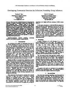
In this subsection, we run EBC, LPAm, SSLM and our method on Karate network, Risk Map network, Collaboration network and one artificial network. Since the community detection results of EBC and LPAm do not change greatly, we give one running result for each of them. SSLM and our method are semisupervised method, the results of them change with the increasing number of labeled nodes. So we do 10 experiments, each experiment use the same method to select different numbers of labeled nodes, and we run our method and SSML 10 times respectively in each experiment. 3.1.1 Zachary’s Network of Karate Club Members Zachary’s network of karate club members [25] is a well-known graph, regularly used as a benchmark to test community detection algorithms (Section 15.1). It consists of 34 vertices, the members of a karate club in the United States, who were observed during a period of three years. Edges connect individuals who were observed to interact outside the activities of the club. At some point, a conflict between the club president and the instructor led to the fission of the club into two separate groups. Indeed, by looking at Fig.1, one can distinguish two aggregations, one around vertices


9

33 and 34 (34 is the president), the other around vertex 1 (the instructor). One can also identify several vertices lying between the two main structures, like 3, 9, 10; such vertices are often misclassified by community detection methods. Fig.1 shows community structure of the network.

21 23

16

19

15

31

27

4 3

2

20

1

9 34 24

8

10

33

30

14

29

18 13 22 6

24252627202122232829132547698111013121514171619183130343332

28 26

32 25

12

11

7

17

5

Fig. 1. Community structure in Karate Club network

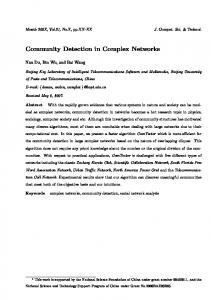
EBC and LPAm wrongly assign the node ’3’ to a community, and the detected community results are the same in different running times. Since the method of selecting nodes is random, the experiments may be different in different running times on the same complex network. We adopt the intermediate result as the result of community detection for SSML on each experiment, and give the worst result on each experiment. Since we use the weighted shortest path to select the labeled nodes, the results of 10 times on each experiment are the same, and they are shown in the Fig.2.

Erro Number of the Nodes

15 Our method SSLM SSLM_Max_Error

10

5

0

2

4

6 8 The number of labeled nodes

10

Fig. 2. Results of Our method and SSML on Karate Club network

Our method reaches a stable state when the number of labeled nodes is larger than 3, and it can rightly divide all the nodes into communities. Although all the

10

nodes can be rightly assigned to communities in the best result of SSML in each experiment, the results of SSML is unstable. Even the numbers of nodes which are wrongly assigned to a community are the same, these nodes are different in different running times, and the performance is not improved with the increasing number of the labeled nodes. SSML Max Error in Fig.2 denotes the worst results of 10 running times on each experiment. 3.1.2 Risk Map Network Risk Map Network was invented by French film director Albert Lamorisse, and was originally released in 1957 in France. Risk is a turn-based game for two to six players. The standard version is played on a board depicting a political map of the Earth, divided into forty-two territories, and these territories are grouped into six continents. The primary object of the game is ”world domination,” or ”to occupy every territory on the board, and in so doing, to eliminate all other players.” Players control armies with which they attempt to capture territories from other players, with results determined by dice rolls. The community structure is shown in Fig.3.

2

6 8

7

9

3

21

13

17

11

14

24

18

23

22

12

15

25

19

27

28

26

16

31 33

34

35

36 37

40

39

42

41

422425262720212223282940411325476983938111013121514171619183130373635343332

32

20

4

10

29 30

1

5

38

Fig. 3. Community structure in Risk Map network

EBC has a better result on Risk Map network compared with LPAm, it wrongly assigns only the nodes ’22’, ’26’ to communities, but LPAm divides this network into 7 communities and wrongly assigns 14 nodes to communities. The experimental results of our method and SSML are shown in the Fig.4. SSML can rightly assign each node to community in the best results when the number of labeled nodes is larger than 7. In this subsection, the intermediate result is viewed as the result of community detection for SSML on each experiment, and the worst results on the 10 experiments are denoted by SSML Max Error in Fig.4. Although the number of the nodes which are wrongly assigned to communities in the detected results of SSML is less than that of our method in some experiments, the worst results of SSML in 10 experiments are all worse than that of our method. At the same time, the community detection results of our method are all the same in 10 running times of each experiment,


11



10

5

0

6

8

10 12 The number of labeled nodes

14

Fig. 4. Results of Our method and SSML on Risk Map Network

this shows that the experimental results of our method is more stable than that of SSML.

3.1.3 Collaboration Network Collaboration network displays the largest connected component of a network depicting collaborations of scientists working at the Santa Fe Institute (SFI). There are 118 vertices, representing resident scientists at SFI and their collaborators. Edges associate with scientists that have published at least one paper together. The visualization layout allows to distinguish disciplinary groups. In this network one observes many cliques, as authors of the same paper are all linked to each other. There are but a few connections between most groups, collaboration network can be divided into 4 communities, and the community structure is shown in the Fig.5.

24252627202122232829488759585554575651505352115114888911111011311282838081861188485371081091021031001011061071041053938333231303736353460616263646566676869269998919093929594979611101312151417161918117 1164849464744454243404115977767574737271707978

Fig. 5. Community structure in Collaboration network

EBC wrongly assigns 32 nodes to a community on collaboration network, this result can not be accepted. The community structure of collaboration network detected by LPAm is worse than that of EBC, LPAm divides collaboration

12

network into 21 communities. The detecting results of our method and SSML are shown in Fig.6.



30 25 20 15 10 5 0

16

18 20 22 The number of labeled nodes

24

Fig. 6. Results of Our method and SSML on Collaboration network

Our method can reach a stable state when the number of labeled nodes is larger than 19, and it wrongly assigns only one node to a community. Although the best results of SSML has no nodes be wrongly assigned to communities when the number of labeled nodes is larger than 17, the worst result in each experiment has too many nodes to be wrongly assigned to communities compared with our method. SSML wrongly assigns more than 15 nodes to communities in more than 6 experiments. In a large complex network, its information of community structure is unknown, we almost have no way to determine which community detection result is better than the rest of results. So in the real application, a stable community detection algorithm should be chosen to detecting the community structure of the large complex networks.

3.1.4 LFR benchmark network LFR benchmark networks [27] are popular used in testing the performance of community detection algorithm. We generate a networks with 1000 nodes. The minimum community has 43 nodes, and the maximum community contains 214 nodes. We run our community detection algorithms, EBC, LPAm and SSML many times. Since the community structure of this network is clear, EBC and LPAm rightly assign all nodes to communities. Our method also can assigns all nodes to right communities when the number of selected nodes is larger than 10. Since SSML adopts random method to select nodes as labeled nodes, if some communities has no nodes to be selected, then the nodes in these communities will be assigned to other communities. Although SSML can assign all nodes to right communities in the best experimental results, the numbers of the nodes which are assigned to wrong communities in the worst result on each experiment are 113, 45, 180, 119, 77, 44, 48, 48, 108, 120 when the numbers of selected nodes are 30, 35, 40, 45, 50, 55, 60, 65,70, 75. These experiments show also show that SSML is an unstable algorithm.


3.2

13

Evaluation with Modularity

The modularity greedy algorithm, originally is described by Newman [27], ranges from 0 to 1. The modularity is viewed as a index to quantify how good a particular division of a network is, a larger value of modularity implies a better division of a complex network. Let eij be one-half of the fraction of edges in the network that connect vertices in group i to those in group j. eii , which are equal to the fraction of edges that fall within group i. The modularity is is described as, ∑ Q= (eii − a2i ) (5) i

where ai is the ∑ fraction of all ends of edges that are attached to vertices in group i, and ai = j eij . Since the performances of ECB and PLAm on Karate, Risk Map and Collaboration network are worse than that of SSML and our method, and ECB, LPAm and our algorithm rightly assigned all the nodes to communities on the artificial network, we only compare our method with SSML on Karate, Risk Map and Collaboration network. The modularity information of our method and SSML on 10 experiments are shown in table 1. nw1 is Zacharys Network of Karate Club Members, nw2 is Risk Map network, nw3 is Collaboration and A1 is our community detection algorithm in Table 1. Table 1. The modularity information of our method and SSML on 10 experiments data Algor A1 nw1 SSML A1 nw2 SSML A1 nw3 SSML

exp1 0.133 0.294 0.596 0.628 0.676 0.666

exp2 0.355 0.303 0.610 0.631 0.676 0.678

exp3 0.372 0.298 0.610 0.617 0.676 0.678

exp4 0.372 0.352 0.610 0.587 0.676 0.677

exp5 0.372 0.355 0.610 0.629 0.677 0.677

exp6 0.372 0.358 0.610 0.608 0.677 0.677

exp7 0.372 0.345 0.622 0.621 0.677 0.677

exp8 0.372 0.360 0.622 0.621 0.677 0.677

exp9 0.372 0.372 0.622 0.623 0.677 0.677

exp10 0.372 0.358 0.622 0.610 0.677 0.677

Table 1 shows that the modularities of our method are larger than that of SSML on the three networks in most of the experiments, and the number of nodes which are wrongly assigned to communities by running our method is less than that of SSML in most of the experiments, and this is also shown in Fig 2. SSML has different modularities which are shown with bold in table 1 when the number of nodes wrongly assigned to communities is the same in different experiments, and this shows that the nodes wrongly assigned to communities are different even the number of them are the same. Although our method wrongly assigns ’26’, ’33’, ’34’ to communities since the seventh experiment on Risk Map network, the node ’26’ can be assigned to any one of three communities based on the ties in Fig 3, and thus the nodes ’33’ and ’34’ are wrongly assigned to communities because of the same reason, and this leads that the modularities are larger than that of the first six experiments. The modularity of our method will not change when our algorithm achieves its stable state, but the modularity of SSML has not any stable value.

14

4

Conclusion and Future Work

In this paper, we introduce active learning method into community detection, and present an algorithm, named active semi-supervised community detection algorithm with label propagation. We select nodes from the core nodes actively using the weighted shortest path and view them as labeled nodes, and experimential results show that the nodes selected by using this method can cover as many communities as possible, and thus we can obtain a stable community detection algorithm. Our community detection algorithm expands the labeled nodes by labeling the neighbors of labeled nodes with a threshold which is obtained automatically based on the characters of the networks. We demonstrate our algorithm with three real networks and one artificial network with wellknown community structures. Althogh our algorithm has a better performance and more stable results compared with SSML, the time complexity is high, especially for the selecting method, algorithm 1. We will research on method of selecting nodes with lower time complexity in the future. Acknowledgments. This paper is Supported by the Fundamental Research Funds for the Central Universities (lzujbky-2012-212).

References 1. Grvan,M., Newman, M.E.J.: Community Structure in Social and Biological Networks.Proc. Natl. Acad. Sci. USA. 99, 7821-7826(2002) 2. Brandes,U.:On Variants of Shortest-path Betweenness Centrality and Their Generic Computation. Social Networks.30,136-145(2008) 3. Newman,M.E.J., Girvan,M.:Finding and Evaluating Community Structure in Networks. Phys. Rev. E. 69, 026113(2004) 4. Comellas,F., Miralles,A.:A Fast and Efficient Algorithm to Identify Clusters in Networks. APPL MATH COMPUT. 217, 2007-2014(2010) 5. Brandes,U., Delling,D., Gaertler,M., G¨ orke, R., Hoefer,M., Nikoloski,Z., Wagner,D.:On Finding Graph Clusterings with Maximum Modularity. In:Proceedings of the 33rd International Workshop on Graph-Theoretic Concepts in Computer Science, LNCS. 4769,121-132 (2007) 6. Chen,W., Liu,Z., Sun,X., Y. Wang.: A Game-theoretic Framework to Identify Overlapping Communities in Social Network. Data Min. Knowl. Discov. 21, 224240(2010) 7. Raghavan, U.N., R. Albert, S. Kumara.: Near Linear Time Algorithm to Detect Community Structures in Large-scale Networks. Phys. Rev. E. 76, 036106(2007) 8. Liu, X., Murata, T.: How Does Label Propagation Algorithm Work in Bipartite Networks? In: IEEE/WIC/ACM International Joint Conference on Web Intelligence and Intelligent Agent Technology, pp. 5-8. IEEE CPS Press, Piscataway (2009) 9. Barber, M. J., Clark, J. W.: Detecting Network Communities By Propagating Labels Under Constraints. Phys. Rev. E. 80, 026129 (2009) 10. Liu, X., Murata, T.: Advanced Modularity-Specialized Label Propagation Algorithm for Detecting Communities in Networks. Physica A. 389, 1493-1500 (2010)


15

11. Xie, J., Szymanski, B.K.: Community Detection Using a Neighborhood Strength Driven Label Propagation Algorithm. In: 1st International Network Science Workshop, pp. 188-195. IEEE CPS Press, Piscataway (2011) ˇ M. Bajec. Unfolding Network Communities by Combining Defensive 12. L. Subelj, and Offensive Label Propagation. In: International Workshop on the Analysis of Complex Networks, pp. 87-104. Catalonia (2010). 13. Ma, X., Gao, L., Yong, X., Fu, L.: Semi-Supervised Clustering Algorithm for Community Structure Detection in Complex Networks. Physica A. 389(1), 187-197 (2010) 14. Silva, T.C., Zhao, L.: Semi-Supervised Learning Guided by The Modularity Measure in Complex Networks. Neurocomputing 78(1), 30-37 (2012) 15. Scheffer, T., Wrobel, S.: Active Learning of Partially Hidden Markov Models. In: 12th ECML/PKDD Workshop on Instance Selection, pp. Freiburg(2001). 16. Melville, P., Mooney, R.J.: Diverse Ensembles for Active Learning. In: 21st International Conference on Machine learning, pp. 584-591. ACM Press, New York (2004) 17. Dasgupta, S., Hsu, D., Monteleoni, C.: A General Agnostic Active Learning Algorithm. In Advances in Neural Information Processing Systems. 353-360 (2008) 18. Nguyen, H. T., Smeulders, A.: Active Learning Using Pre-Clustering. Proceedings of the twenty-first international conference on Machine learning. 623-630 (2004) 19. Vu, V.V., Labroche, N., Meunier, B.B.: Active Learning for Semi-Supervised KMeans Clustering. In: 22nd International Conference on Tools with Artificial Intelligence, pp. 12-15. IEEE CPS Press, Piscataway (2010) 20. Zhao, W., He, Q., Ma, H., Shi, Z.: Effective Semi-Supervised Document Clustering Via Active Learning with Instance-Level Constraints. KNOWL INF SYST. 30(3), 569-587 (2012) 21. Grira, N., Crucianu, M., Boujemaa, N.: Active Semi-Supervised Fuzzy Clustering. PATTERN RECOGN. 41(5), 1834-1844(2008) 22. Wang, X., Davidson, I.: Active Spectral Clustering. 2010 IEEE International Conference on Data Mining. 561-568 (2010) 23. Mallapragada, P. K., Jin, R., Jain, A. K.: Active Query Selection for SemiSupervised Clustering. In: 19th International Conference on Pattern Recognition, pp. 1-4. IEEE Press, Piscataway (2008) 24. Huang, R., Lam, W., Zhang, Z.: Active Learning of Constraints for SemiSupervised Text Clustering. In: 7th SIAM International Conference on Data Mining, pp. 113-124. Society for Industrial and Applied Mathematics Publications Press, Philadelphia (2007) 25. Zachary, W.W.: An Information Flow Model for Conflict and Fission in Small Groups, J. Anthropol. Res. 33(4), 452-473 (1977) 26. http://en.wikipedia.org/wiki/Risk (game) 27. Lancichinetti, L., Fortunato, F., Radicchi,R.: Benchmark graphs for testing community detection algorithms. Phys. Rev. E.78, 046110 (2008) 28. Newman, M.E.J.: Fast Algorithm for Detecting Community Structure in Networks. Phys. Rev. E. 69, 066133 (2004)