Active Shape Models with Invariant Optimal Features (IOF-ASMs). Federico Sukno1,2, Sebastián Ordás1, Costantine Butakoff1,. Santiago Cruz2, and Alejandro ...
365
Active Shape Models with Invariant Optimal Features (IOF-ASMs) Federico Sukno1,2 , Sebasti´ an Ord´ as1 , Costantine Butakoff1 , 2 Santiago Cruz , and Alejandro Frangi1 1 2
Department of Technology, Pompeu Fabra University, Barcelona, Spain Aragon Institute of Engineering Research, University of Zaragoza, Spain
Abstract. This paper is framed in the field of statistical face analysis. In particular, the problem of accurate segmentation of prominent features of the face in frontal view images is addressed. Our method constitutes an extension of Cootes et al. [6] linear Active Shape Model (ASM) approach, which has already been used in this task [9]. The technique is built upon the development of a non-linear appearance model, incorporating a reduced set of differential invariant features as local image descriptors. These features are invariant to rigid transformations, and a subset of them is chosen by Sequential Feature Selection (SFS) for each landmark and resolution level. The new approach overcomes the unimodality and gaussianity assumptions of classical ASMs regarding the distribution of the intensity values across the training set. Validation of the method is presented against the linear ASM and its predecesor, the Optimal Features ASM (OF-ASM) [14] using the AR and XM2VTS databases as testbed.
1
Introduction
In many automatic systems for face analysis, following the stage of face detection and localization and before face recognition is performed, facial features must be extracted. This process currently occupies a large area within computer vision research. A human face is part of a smooth 3D object mostly without sharp boundaries. It exhibits an intrinsic variability (due to identity, gender, age, hairstyle and facial expressions) that is difficult if not impossible to characterize analytically. Artifacts such us make-up, jewellery and glasses cause further variation. In addition to all these factors, the observer’s viewpoint (i.e. in-plane or in-depth rotation of the face), the imaging system, the illumination sources and other objects present in the scene, affect the overall appearance. All these intrinsic and extrinsic variations make the segmentation task difficult and discourage a search for fixed patterns in facial images. To overcome these limitations, statistical learning from examples is becoming popular in order to characterize, model and segment prominent features of the face. An Active Shape Model (ASM) is a flexible methodology that has been used for the segmentation of a wide range of objects, including facial features [9]. In T. Kanade, A. Jain, and N.K. Ratha (Eds.): AVBPA 2005, LNCS 3546, pp. 365–375, 2005. c Springer-Verlag Berlin Heidelberg 2005 �
366
Federico Sukno et al.
the seminal approach by Cootes et al. [6] shape statistics are computed from a Point Distribution Model (PDM) and a set of local grey-level profiles (normalized first order derivatives) is used to capture the local intensity variations at each landmark point. In [5] Cootes et al. introduced another powerful approach to deformable template models, namely the Active Appearance Model (AAM). In AAMs a combined PCA of the landmarks and pixel values inside the object is performed. The AAM handles a full model of appearance, which represents both shape and texture variation. The speed of ASM-based segmentation is mostly based on the simplicity of its texture model. It is constructed with just a few pixels around each landmark whose distribution is assumed to be gaussian and unimodal. This simplicity, however, becomes a weakness when complex textures must be analyzed. In practice, its local grey-levels around the landmarks can vary widely and pixel profiles around an object boundary are not very different from those in other parts of the image. To provide a more complete intensity model, van Ginneken et al. [14] proposed an Optimal Features ASM (OF-ASM), which is non-linear and allows for multi-modal intensities distribution, since it is based on a k-nearest neighbors (kNN) classification of the local textures. The main contribution of that approach is an increased accuracy in the segmentation task that has shown to be particularly useful in segmenting objects with textured boundaries in medical images. However, its application to facial images is not straightforward. Facial images have a more complicated geometry of embedded shapes and present large texture variations when analyzing the same region for different individuals. In this work we will discuss those problems and develop modifications to the model in order to make it deal with face complexities, as well as the replacement of the OF-ASM derivatives so that the intensity model is invariant to rigid transformations. The new method, coined Invariant Optimal Features ASM (IOF-ASM) will also attack the segmentation speed problem, mentioned as a drawback in [14]. The performance of our method is compared against both the original ASM and the OF-ASM approaches, using the AR [11] and XM2VTS [12] databases as test bed. Experiments were split into segmentation accuracy and identity verification rates, based on the Lausanne protocol [12]. The paper is organized as follows. In Section 2 we briefly describe the ASM and OF-ASM, while in Section 3 the proposed IOF-ASM is presented. In Section 4 we describe the materials and methods for the evaluation and show the results of our experiments and Section 5 concludes the paper.
2 2.1
Background Theory Linear ASM
In its original form [6], ASMs are built from the covariance matrices of a Point Distribution Model (PDM) and a local image appearance model around each of those points. The PDM consists of a set of landmarks placed along the edges or contours of the regions to segment. It is constructed by applying PCA to the aligned set
Active Shape Models with Invariant Optimal Features (IOF-ASMs)
367
of shapes, each represented by a set of landmarks [6]. Therefore, the original shapes ui and their model representation bi are related by the mean shape u and the eigenvectors matrix Φ: bi = ΦT (ui − u),
ui = u + Φbi
(1)
It is possible to use only the first M eigenvectors with the largest eigenvalues. In that case (1) becomes an approximation, with an error depending on the magnitude of the excluded eigenvalues. Furthermore, under the assumption of gaussianity, each component of the bi vectors is constrained to ensure that only valid shapes are represented: � 1 ≤ i ≤ N, 1 ≤ m ≤ M (2) bm i ≤ β λm where β is a constant, usually set between 1 and 3, according to the degree of flexibility desired in the shape model and λm are the eigenvalues of the covariance matrix. The intensity model is constructed by computing second order statistics for the normalized image gradients, sampled on each side of the landmarks, perpendicularly to the shape’s contour. The matching procedure is an iterative alternation of landmark displacements based on image information and PDM fitting, performed in a multi-resolution framework. The landmark displacements are provided using the intensity model, by minimizing the Mahalanobis distance between the candidate gradient and the model’s mean. 2.2
Optimal Features ASM
As an alternative to the construction of normalized gradients and to the use of the Mahalanobis distance as a cost function, van Ginneken et al. [14] proposed to use a non-linear gray-level appearance model and a set of features as local image descriptors. Again, the landmark points are displaced to fit edge locations during optimization, along a profile perpendicular to the object’s contour at every landmark. However, the best displacement here will be the one for which everything on one side of the profile is classified as being outside the object, and everything on the other side, as inside of it. Optimal Features ASMs (OFASMs) use local features based on image derivatives to determine this. The idea behind that is the fact that a function can be locally approximated by its Taylor series expansion provided that the derivatives at the point of expansion can be computed up to a sufficient order. The set of features is made optimal by sequential feature selection [8] and interpreted by a kNN classifier with weighted voting [3], to hold for non-linearity.
3 3.1
Invariant Optimal Features ASM Multi-valued Neural Network
In our approach we used a non linear classifier in order to label image points near a boundary or contour. In principle, any classifier can be used, as long as it can
368
Federico Sukno et al.
cope with the non-linearity. Between the many available options, our selection was the Multivalued Neural Network (MVNN) [2], mainly based on the need to improve segmentation speed. This is a very fast classifier, since its decision is based only on a vector multiplication in the complex domain. Furthermore, a single neuron is enough to deal with non-linear problems [1], which avoids the need for carefully tuning the number of layers (and neurons in each of them) that characterizes multi-layer perceptron networks. The MVNN will have as many inputs as the number of features selected for each landmark (say NF ), all of them being integer numbers, and a single integer output. The classification is performed by a single neuron, which for every input xk finds a corresponding complex number on the unit circle: qk = exp(j2πxk )
1 ≤ k ≤ NF
(3)
xk being the k-th input variable value (discrete), qk its corresponding complexplane√representation, NF the number of inputs (features) and j the imaginary unit −1. Then, the neuron maps the complex inputs to the output plane by means of the NF -variable function fNF : k k k+1 ) when 2π ≤ arg(z) < 2π NO NO NO z = w0 + w1 q1 + w2 q2 + ... + wNF qNF
fNF (z) = exp(j2π
(4) (5)
where wk are the network weights learnt during the training phase. The fNF ’s image is a complex plane, which has been divided into NO angular sectors, like a quantization of arg(z). In other words, the neuron’s output is defined as the number of the sector in which the weighted sum z has fallen. Notice that the number of sectors of the input and output domains does not need to be the same. 3.2
Irreducible Cartesian Differential Invariants
A limitation of using the derivatives in a cartesian frame as features in the OF-ASM approach is the lack of invariance with respect to translation and rotation (rigid transformations). Consequently, these operators can only cope with textured boundaries with the same orientations as those seen in the training set. To overcome this issue we introduce a multi-scale feature vector that is invariant under 2D rigid transformations. It is known [7][15] that Cartesian differential invariants describe the differential structure of an image independently of the chosen cartesian coordinate system. The term irreducible is used to indicate that any other algebraic invariants can be reduced to a combination of elements in this minimal set. Table 1 shows the Cartesian invariants up to second order. To make our approach invariant to rigid transformations we use these invariants at three different scales, σ = 1, 2 and 4. The zero order invariants were not used since the differential images are expected to provide more accurate and
Active Shape Models with Invariant Optimal Features (IOF-ASMs)
369
Table 1. Tensor and Cartesian formulation of invariants Tensor Formulation L Lii Li Li Li Lij Lj Lij Lji
2D Cartesian Formulation L Lxx + Lyy L2x + L2y L2x L2xx + 2Lxy Lx Ly + L2y L2yy L2xx + L2xy + L2yy
stable information about facial contours (edges). For each landmark and resolution level, a sequential feature selection algorithm [8] was used to reduce the size of the feature vector. In this way, only a subset of the invariants drove the segmentation process. 3.3
Texture Classifiers for IOF-ASM
IOF-ASM is basically an improved OF-ASM. The first two improvements are the new and much faster classifier and the use of features invariant to rigid transformations of the input image. Only one improvement is left that we will be stated below. Let us look back for a moment at OF-ASM. Its training is based on a landmarked set of images for which all of the derivative images are computed and described by local histograms statistics. The idea behind this method is that, once trained, texture classifiers will be able to label a point as inside or outside the region of interest based on the texture descriptors (the features) or, ideally, on a smaller (optimal ) subset of them. Therefore, labelling inside pixels with 1 and outside pixels with 0 and plotting the labels corresponding to the profile pixels, the classical step function is obtained, and the transition will correspond to the landmark position. Nevertheless, there are a couple of reasons why this will not happen. The first one is that certain regions of the object are thinner than the size of the grid, and then the correct labelling of the points will look more like a bar than like a step function. An indicative example arises when the square grid is placed on the eyes or eyebrows contours, especially if using a multiresolution framework, as ASM does (Fig. 1). Another problem is that the classifiers will not make a perfect decision, so the labelling will look much noisier than the ideal step or bar. Moreover, Fig. 1 illustrates how, for certain landmarks where there is a high contour curvature (i.e mouth/eyes/eyebrows corners), most of the grid points lie outside the contour, promoting quite an unbalanced training of the classifiers. To tackle these problems, in our IOF-ASM we introduced new definitions of input and output of the classifiers. For each landmark, instead of the Gaussian weighted histograms used in OF-ASM, we place a square grid, with a subgrid at each cell of the main grid. In other words, in previous approaches fixed positions along the normal were used to sample pixels. We extended this approach and defined a grid with its center on the landmark. Then for each cell of this grid we use a classifier, whose inputs are taken from a subgrid centered at each of the cells of the main grid.
370
Federico Sukno et al.
Fig. 1. A typical eyebrow image and a 5x5 grid with the arrow indicating the normal to the contour (Left); The same grid in the mouth corner, where only 3 points lie inside the lip (Center); and the typical graphs of the profiles for OF- and IOF-ASM (Right)
Regarding the outputs, the bi-valued labelling (inside-outside) is replaced with the distance of the pixels to the landmarked contour. Then, for each cell of the main grid the classifiers are trained to return the distance to reach the landmark. Since those centers are placed along normals to the contour, the typical plot of the labels will take a shape of letter ”V”, with its minimum (the vertex) located at the landmark position, irrespective of which region is sampled or its width relative to the grid size. At matching time, this labelling strategy allows for introducing a confidence metric. The best position for the landmark is now the one which minimizes the profile distance to the ideal ”V” profile, excluding the outliers. An outlier here is a point on the profile whose distance to the ideal one is greater than one. It can be easily understood by noticing that such a point is suggesting a different position to place the landmark (i.e. its distance would be smaller if the V is adequately displaced). If the number of outliers exceeds 1/3 of the profile size, then the image model is not trustworthy and the distance for that position is set to infinity. Otherwise, preference is given to the profiles with fewer outliers. The function to minimize is: f (k) = NOL +
1 NP − NOL
−NOL NP�
|pi − vi |
(6)
i=1
where k are the candidate positions for the landmark, NOL is the number of outliers, NP the profile size, and p and v are the input and ideal (V) profiles, respectively.
4
Experiments
The performance of the proposed method was compared with the ASM and OF-ASM schemes. Two datasets were used. The first one is a subset of 532 images from the AR database [11], showing four different facial expressions of 133 individuals. This database was manually landmarked with a 98-point PDM template that outlines the eyes, eyebrows, nose, mouth and face silhouette. The second dataset is the XM2VTS [12] database, composed of 2360 images (8 for each of 295 individuals).
Active Shape Models with Invariant Optimal Features (IOF-ASMs)
371
Fig. 2. Mean fitting error performance in 532 frontal images of the AR database
Both segmentation accuracy and identity verification scores have been tested. In order to make verification scores comparable between the two datasets, the AR images were divided into five groups, preserving the proportions of the Lausanne Protocol [12] (configuration 2) for the XM2VTS database. In this way, we came out with 90 users (two images/each for training, one for evaluation and one for testing), 11 evaluation impostors (44 images) and 32 test impostors (128 images). It must be pointed out that the individuals on each group were randomly chosen, making sure that there is the same proportion of men/women in all of them. Moreover, they are also balanced in the amount of images per facial expression. 4.1
Segmentation Accuracy
The segmentation accuracy was tested on the AR dataset only, since this task needs the input images to be annotated. For the same reason, all models constructed in our experiments were based on the Training Users group of the AR dataset. Table 2 summarizes the parameters used by the 3 compared models. Additionally, we use 150 PCA modes for the PDM, β = 1.5 (see (2)) and a search range of ±3 pixels along the profiles at each resolution. The segmentation results are displayed in Fig. 2. The displayed curves show the mean Euclidean distance (± the standard error) between the segmentation using the corresponding model and the manual annotations for each landmark, normalized as a percentage of the distance between the true centers of the eyes. The mean eyes-distance in the AR dataset is slightly greater than 110 pixels, so the curves give the fitting error approximately in pixel units.
372
Federico Sukno et al. Table 2. Parameters used to build the statistical models Parameter Profile length Grid size Each grid point Resolutions Selected features
ASM 8 n/a n/a 4 n/a
OF-ASM n/a 5×5 α = 2σ 5 6 of 36 15
8 7 6 5
10
4 ASM matching IOF−ASM matching PCA reconstruction
3 2 1 1
OF−ASM ASM IOF−ASM
Mean fitting error +/− standard error
Mean fitting error +/− standard error
9
IOF-ASM 7 7×1 7 × 5 patch 5 70 of 420
1.1
1.2
1.3 1.4 1.5 1.6 1.7 PDM flexibility (Beta)
1.8
1.9
2
5 −60
−40
−20 0 20 40 Images rotation angle (degrees)
60
Fig. 3. Segmentation errors vs. PDM flexibility (Left) and vs. rotation angles of the input images (Right)
It is clear from Fig. 2 that OF-ASM produces a segmentation error significantly larger than the other methods, due to the problems that were previously discussed, mainly regarding shape complexity. On the other hand, IOF-ASM outperforms ASM in all regions, and the difference is statistically significant in several landmarks. The average improvement of IOF-ASM with respect to the ASM segmentation is of 13.2%, with a maximum and minimum of 28.5% and 5.2% in the eyes and silhouette contour respectively. Fig. 3 (Left) shows further comparison of ASM and IOF-ASM accuracy when varying the PDM flexibility parameter β (see (2)). It can be seen that as β increases, the difference between the error of both models tends to grow. At the same time, the PCA reconstruction error introduced by the PDM decreases, so the segmentation relies more on the image model precision. This behavior enforces the hypothesis of performance improvement in favor of IOF-ASM. The three models are always initialized with their mean shape centered at the true face centroid (according to the annotations) and scaled to 80% of the mean size of the faces in the database. Notice in Table 2 that the image model search range for all models is ±3 pixels per resolution level, giving a total of ±3 × 2NR−1 pixels, for NR resolutions. Considering such initialization, the initial distance between the model landmarks and the annotated positions will be up to 68 pixels in the lower lip and the chin, and up to 40 pixels in the rest of the face, so NR should be fixed at least to 5. However, in our experiments the best performance for ASM was obtained with 4 resolutions, and therefore we used this value.
Active Shape Models with Invariant Optimal Features (IOF-ASMs)
373
Table 3. Identity Verification Scores
4.2
Database AR
Set Evaluation Test
XM2VTS
Evaluation Test
Parameter EER FAR FRR EER FAR FRR
ASM 3.3% 3.6% 3.3% 11.0% 10.9% 12.8%
IOF-ASM 3.3% 3.9%