3D Active Shape Model Segmentation with

3D Active Shape Model Segmentation with Nonlinear Shape Priors Matthias Kirschner, Meike Becker, and Stefan Wesarg Graphisch-Interaktive Systeme, Technische Universit¨ at Darmstadt, Fraunhoferstraße 5, 64283 Darmstadt, Germany {matthias.kirschner,meike.becker,stefan.wesarg}@gris.tu-darmstadt.de

Abstract. The Active Shape Model (ASM) is a segmentation algorithm which uses a Statistical Shape Model (SSM) to constrain segmentations to ‘plausible’ shapes. This makes it possible to robustly segment organs with low contrast to adjacent structures. The standard SSM assumes that shapes are Gaussian distributed, which implies that unseen shapes can be expressed by linear combinations of the training shapes. Although this assumption does not always hold true, and several nonlinear SSMs have been proposed in the literature, virtually all applications in medical imaging use the linear SSM. In this work, we investigate 3D ASM segmentation with a nonlinear SSM based on Kernel PCA. We show that a recently published energy minimization approach for constraining shapes with a linear shape model extends to the nonlinear case, and overcomes shortcomings of previously published approaches. Our approach for nonlinear ASM segmentation is applied to vertebra segmentation and evaluated against the linear model.

1

Introduction

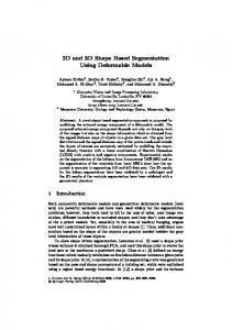
Accurate segmentation of organs in medical images is challenging, because adjacent structures are often mapped to the same range of intensity values, which makes it hard to detect their boundaries. In these cases, prior knowledge of the shape of an organ can be used to avoid that the segmentation leaks into the neighboring structures. One of the most popular segmentation algorithms with a shape prior is the Active Shape Model (ASM) [1], which uses a linear, landmark-based Statistical Shape Model (SSM). The linear SSM is learned by a Principal Component Analysis (PCA) of the training shapes, which implies the assumption that the shapes are Gaussian distributed. While this model has been successfully applied to the segmentation of various structures in medical imaging, there are cases in which the assumption does not hold true. An example for such a case is shown in Figure 1 (left), which shows a training data set consisting of 14 lumbar (L1-L3) and 9 thoracic (Th10Th12) vertebrae, projected to the first two principal components. One can clearly see that each vertebra type (thoracic, lumbar) builds a cluster. The mean shape of this training data set shows characteristics of both lumbar and thoracic shapes

2

Matthias Kirschner, Meike Becker, Stefan Wesarg

Fig. 1. Left: A set of 14 lumbar vertebrae (green triangles) and nine thoracic vertebrae (blue circles), projected to the first two principal components. The shading encodes values of the log-likelihood function of the learned Gaussian. The brighter the shading, the higher is the probability. The curves show isocontours of the function. Right: The mean shape, which shows characteristics of both lumbar and thoracic vertebrae.

(Figure 1, right). While it is the most likely shape with respect to the linear SSM, we would not expect a vertebra of this shape in the human body. To describe such datasets more accurately, nonlinear, multimodal models are required. Several nonlinear extensions of SSMs for ASM segmentation have been proposed in the literature, for example based on Kernel Principal Component Analysis (KPCA) [2, 3] or Gaussian Mixture Models [4]. However, to the best of our knowledge, these approaches have never been applied to segmentation in 3D, which typically suffers from the huge gap between the high dimensionality of the shapes and the small number of training examples. In fact, Heimann and Meinzer observe in their recent review [5] that nonlinear, landmark-based SSMs have hardly attracted the attention of the community so far. This stands in contrast to level set segmentation with shape priors, where nonlinear techniques such as KPCA [6] or Parzen Density estimation [7] are becoming increasingly popular for learning priors from signed distance functions. In this paper, we take a first step towards bridging the gap between theoretical models on one side and real world applications on the other. We summarize our main contributions as follows: 1. We discuss methodological shortcomings of previously published approaches for constraining shapes in nonlinear ASMs, especially in the case of high dimensional training data sets with few training examples. 2. We present a unified formulation for constraining shapes in ASMs, which contains linear shape models as special cases. 3. We present a particular nonlinear ASM based on KPCA (KPCA-ASM). 4. We apply the KPCA-ASM to the real world problem of segmenting vertebrae in 3D CT scans. Our evaluation provides insights into the properties of the nonlinear ASM, and shows that it can increase the segmentation accuracy in certain applications.

3D Active Shape Model Segmentation with Nonlinear Shape Priors

2

3

Statistical Shape Models and the Active Shape Model

In this section, we briefly review Statistical Shape Models (SSM) and the segmentation algorithm Active Shape Model (ASM), which were both introduced by Cootes et al. [1]. In SSMs, each of the S training shapes is represented by (j) N corresponding landmarks xi = (xij , yij , zij ), which are concatenated to the shape vector xi = (xi1 , yi1 , zi1 , . . . , xiN , yiN , ziN ) ∈ IR3N . Procrustes alignment is used to compute a common coordinate system for the shapes. The linear SSM uses PCA to capture the statistics of the training shapes. One computes the eigenvectors p1 , . . . , p3N andP corresponding eigenvalues λ1 ≥ . . . ≥ λ3N of the S 1 covariance matrix C = S−1 ¯)(xi − x ¯)T of the shapes. We discard i=1 (xi − x P3N P t′ eigenvectors with index i > t, were t = min{t′ | i=1 λi / i=1 λi > 0.98}. The 3N × t-matrix of retained eigenvectors is denoted by P = (p1 | . . . |pt ), and the subspace of IR3N spanned by these eigenvectors is denoted by U . The ASM is an iterative algorithm, which is initialized by placing the mean shape into the image. Each iteration consists of two steps: Landmarks are displaced to optimal image features in their vicinity, which have been selected by an appearance model. Then the deformed shape is constrained with the SSM.

3

Shape constraints for linear and nonlinear ASMs

In the original ASM algorithm, a shape x′ is constrained to a plausible shape x (a) by projecting x′ to U using the formula b = P T (x′ − x ¯),

(1)

(b) √ by imposing bounds on the subspace vector b, e. g. by enforcing that bi ∈ √ [−3 λi , 3 λi ], and (c) by generating the plausible shape by x = x ¯ + P b. This approach cannot be trivially extended to nonlinear shape models. For example, Romdhani et al. [2] place upper bounds on the KPCA components like in the linear model, but it has been shown that this approach is not valid in general [3]. Instead, Cootes et al. [4] and Twining and Taylor [3] propose to constrain shapes with nonlinear shape models by minimizing an energy Eshape (x) until Eshape (x) ≤ θ, where θ defines a plausibility threshold. In contrast to the least squares projection in Eq. 1, this approach does not guarantee a result which is close to the deformed shape x′ . Furthermore, it restricts the space of allowed shapes to those shapes which are close to the isocontour Eshape (x) = θ, and it remains open how to choose θ. Finally, the ‘proximity to data’ measure for KPCA [3] does not penalize the possible loss of information that may occur when projecting to a feature space. This loss can be considerably high, especially in case of high dimensional shapes and small training data sets. A unified approach for constraining shapes: The first two of the aforementioned problems can be solved by adding an image energy Eimage (x) that penalizes deviations from the boundary detected by the appearance model. A

4


Fig. 2. Visualization of two KPCA-based shape energies (Left: σ3 ; Right: σ9 ). In contrast to the Gaussian energy (Figure 1), these energies are multimodal.

deformed shape x′ is constrained by minimizing E(x) = α·Eimage (x)+Eshape (x) until a (possibly local) minimum is reached. The parameter α balances image and shape energy, and must be chosen appropriately. In order to account for the loss of information that occurs when projecting to a feature space, we use the general approach of Moghaddam and Pentland [8]: The shape energy is split into two terms, namely the distance in feature space (DIFS) and the distance from feature space (DFFS). The DIFS computes the probability in feature space, whereas the DFFS penalizes the costs of the projection to the feature space. In the linear case, the feature space is U , and the energy becomes 1 X b2i 1 + krk2 , 2 i=1 λi 2ρ t

Eshape−pca (x) =

(2)

where krk2 = kx − x ¯k2 − kbk2 is the costs of the projection of x to U , and P3N ρ = i=t+1 3Nλi−t . We have recently shown [9] that an ASM based on this energy has better segmentation accuracy than the standard approach which uses Eq. 1 as it is less restrictive: By using the DFFS, shapes can leave the subspace U . It permits a limited amount of variability that has not been previously observed in the training data, such that the model adapts better to unseen shapes. KPCA shape energy: KPCA [10] is a nonlinear extension of PCA: The basic principle is to map the input data to a feature space F and subsequently do a linear PCA of the mapped data. The mapping is implicitly defined by a kernel func2 tion k(x, y). We use a Gaussian kernel function k(x, y) = exp − kx−yk 2σ 2 , where the parameter σ controls P the width of the kernel. The centered kernel is defined PS P S S ˜ by k(x, y) = k(x, y) − S1 i=1 (k(x, xi ) + k(y, xi )) + S12 i=1 j=1 k(xi , xj ). In order to do KPCA of the training shapes, we first compute the Gram ˜ i , xj ), and then determine the matrix K ∈ IRS×S with the entries K ij = k(x eigendecomposition of K, which yields its eigenvectors a1 , . . . , aS and eigenvalues ν˜1 , . . . , ν˜S . We introduce a regularization parameter ǫ˜ = 0.001 and discard all eigenvectors with ν˜i ≤ ǫ˜. The remaining r eigenvectors are re-normalized such −1 1 1 that ν˜i 2 aTi a = 1. Moreover, we define νi = S−1 ν˜i and ǫ = S−1 ǫ˜.


The r KPCA components of x can be computed by βi = The shape energy for a KPCA shape model is defined by Eshape−kpca (x) =

t X β2

t X 1 ˜ βi2 ). + (k(x, x) − νi ǫ i=1 i

i=1

PS

j=1

5

˜ i , x). aij k(x

(3)

Note the similarity between Eq. 3 and Eq. 2. In fact, the above definitions are designed so that in the case of ǫ = ρ and klin (x, y) = xT y, both energies are identical up to a constant factor of 2. We want to mention that Eq. 3 has been previously used by Cremers et al. [11] in a Mumford-Shah based level set segmentation system. However, to the best of our knowledge, it has never been used in an ASM. Instead of evolving a curve, we find a local minimum of the combined image and shape energy in each ASM iteration. We use the L-BFGS method [12] to minimize the energy, which is designed for high-dimensional problems. Figure 2 visualizes two instances of the function Eshape−kpca (x), learned from the vertebral shape data set.P We used here the Gaussian kernel with widths σ3 S and σ9 , where σK = K · S1 i=1 minj∈{1,...,S} kxi − xj k, a choice inspired by Cremers et al. [11]. In both cases, the KPCA shape energies are multimodal, in contrast to the linear shape energy (Figure 1), which has a single peak in a region which is not occupied by any training examples. Enforcing smoothness: A high image energy and a high ρ or ǫ permits larger deviations from the training shapes. While additional flexibility of the SSM is certainly desired, because it allows for more accurate segmentations, no force controls the nature of this deformation. This means that individual landmarks can be drawn towards outliers of the appearance model, and the segmentations become jagged. We therefore explicitly enforce smooth segmentations by smoothing the shape after energy minimization with a Laplacian filter: Let q be the position of a landmark, and let m be the mean of its neighbors. We move q to m if kq − mk > 1.2 · δq . For each landmark, the constant δq is set to the maximal distance between q and m in the training data. In each ASM iteration, we iterate five times through all landmarks in order to smooth the shape.

4

Appearance Model and Image Energy

Klinder et al. [13] achieve good segmentation results for vertebrae with an appearance model that considers the image intensity, gradient magnitude and gradient direction. While their model uses various ad-hoc parameters, we combine these features in a more principled, purely statistically motivated way. Each image feature vector sampled at a boundary voxel v consists of a five dimensional feature vector f = (I(v), kG(v)k, G1 (v), G2 (v), G3 (v)). Here, I(v) is the image intensity at voxel v, G(v) = (G1 (v), G2 (v), G3 (v)) is the gradient and kG(v)k its magnitude. In our implementation, G(v) is computed in normal direction n of the current landmark. We compute an orthonormal basis {n, n′ , n′′ }, and use

6


these directions to compute G(v) with finite differences, instead of using the image axes. We model the distribution of f by the product of two independent probability distributions: A Gaussian distribution over f 1 = (I(v), kG(v)k) with mean µ and covariance matrix Σ, and a Fisher distribution [14] over f 2 = G(v) with mean η and concentration parameter κ. This motivates our fitness function g(f ) = − 12 (f 1 − µT )Σ −1 (f 1 − µ) + κ · f T2 η − κ, which is the log-likelihood of the assumed distribution up to a constant term. We have g(f ) ≤ 0 for all f . The parameters Σ, µ, κ and η are PNlearned from the training data. We define the image energy by Eimage (x) = j=1 (1 − g(f (j) ))−1 kx(j) − x′(j) k2 , where x′ is the deformed shape and f (j) the feature at landmark j.

5

Experiments

In our evaluation, we used seven CT scans of the abdomen from a publicly available database1 . We manually segmented the vertebrae in these scans, and used the data from the first five scans as training data and the remaining as test data. All in all, the training data set consists of nine thoracic (Th10: 1; Th11: 3; Th12: 5) and 14 lumbar (L1: 5; L2: 5; L3: 4) vertebrae. The test data set consists of five thoracic (Th10: 1; Th11: 2; Th12: 2) and six lumbar (L1: 2; L2: 2; L3: 2) vertebrae. In the experiments, we segmented the test data with three different types of ASMs: The standard linear ASM, the linear ASM with energy minimization [9], and the KPCA-ASM with different kernel widths. Dependent on the chosen shape model, the shape energy returns different numerical values, which made it necessary to balance α for each method individually in order to achieve good segmentation results. This was done manually by trying different values for α and bracketing the optimal choice. Initial pose parameters of the SSM were determined manually for each test data set. The same manual initialization was used for each tested approach. Each ASM was executed for 50 iterations. We evaluated the segmentation quality with the measures Volumetric Overlap Error (VOE), Average Surface Distance (ASD), and Hausdorff Distance (HD) (see [15] for definitions). 1

3D-IRCADb-01: http://www.ircad.fr/softwares/3Dircadb/3Dircadb1/

Table 1. Segmentation results obtained with different ASM algorithms. The table shows average results and standard deviations (SD).

Manual Initialization Linear ASM (standard) Linear ASM (α = 2000) KPCA-ASM (σ3 , α = 1750) KPCA-ASM (σ6 , α = 100) KPCA-ASM (σ9 , α = 50)

VOE [%] 60.66 SD: 7.01 22.33 SD: 6.55 20.38 SD: 7.62 17.40 SD: 6.66 17.55 SD: 3.80 17.45 SD: 4.14

ASD [mm] 3.83 SD: 0.82 0.83 SD: 0.33 0.73 SD: 0.38 0.61 SD: 0.32 0.60 SD: 0.22 0.60 SD: 0.22

HD [mm] 16.40 SD: 2.97 7.99 SD: 3.41 7.27 SD: 3.64 7.95 SD: 3.52 6.88 SD: 2.45 6.95 SD: 2.72


7

Fig. 3. Comparison of segmentation results for a thoracic vertebra (Th11): The linear ASM cannot always separate ribs and vertebra (left). The KPCA-ASM has more specific shape constraints, and separates vertebra and ribs well (right).

6

Results

The quantitative results of our experiments are shown in Table 1. It can be seen that the KPCA-ASMs outperform the linear ones. Compared to the standard linear ASM, the VOE decreases by over 20 %, the ASD by more than 25 %. Depending on σ, the HD decreases by up to 13 %. The increase of accuracy is especially large for thoracic vertebrae, where the average HD decreases by more than 20 % from 8.7 mm (standard ASM) to 6.8 mm (KPCA-ASM σ6 ). A qualitative result for a thoracic vertebra is shown in Fig. 3. The standard ASM required 13 seconds, and the KPCA-ASM between 40 and 65 seconds.

7

Discussion

In this paper, we presented a unified approach for constraining linear and nonlinear shapes in ASMs. Based on this model, we devised a nonlinear KPCA-ASM, which we used for segmenting vertebrae in CT scans. Our evaluation clearly shows that a KPCA-ASM can increase the segmentation accuracy compared to linear ASMs in applications where the training data has a nonlinear distribution. In our opinion, the reason for this is that the KPCA-ASM is more specific than the linear ASM, and thus detects outliers of the appearance model more effectively. While the nonlinearity of our training data is obvious, because it can be separated into lumbar and thoracic vertebrae, the nonlinear structure of the data may be more subtle in other cases. However, our nonlinear SSM was trained in a completely unsupervised way, without prior knowledge about clusters. This is why we expect that a KPCA-ASM will also perform well in other scenarios with nonlinearly distributed training data. Compared to the results recently reported by Klinder et al. [13], we achieve a significantly better ASD for segmenting individual vertebrae, although it must be mentioned that we have used manual initialization here. Note that Klinder et al. first try to identify the vertebra (e. g. L1), and then segment it with models

8


dedicated to this vertebra. Our quantitative results indicate that, given a reasonably well initialization, the KPCA-ASM is able to automatically determine the correct vertebra class during segmentation. A drawback of the KPCA-ASM is that several parameters must be chosen, such as the kernel width σ, the regularization parameter ǫ˜ and the image energy force α. However, our evaluation shows that the effort for tuning pays off. To the best of our knowledge, this is the first time that a nonlinear ASM has been successfully applied to the segmentation of organs in tomographic 3D scans. Given the positive evaluation results of our study, we expect that nonlinear ASMs will play an important role in medical image segmentation in the future.

References 1. Cootes, T.F., Taylor, C.J., Cooper, D.H., Graham, J.: Active shape models - their training and application. Comput Vis and Image Underst 61(1) (1995) 38–59 2. Romdhani, S., Gong, S., Psarrou, A.: A multi-view nonlinear active shape model using kernel PCA. In: BMVC’99. (1999) 483–492 3. Twining, C.J., Taylor, C.J.: Kernel principal component analysis and the construction of non-linear active shape models. In: BMVC 2001. (2001) 4. Cootes, T.F., Taylor, C.J.: A mixture model for representing shape variation. In: Image and Vision Computing. (1997) 110–119 5. Heimann, T., Meinzer, H.P.: Statistical shape models for 3D medical image segmentation: A review. Medical Image Analysis 13(4) (2009) 543–563 6. Dambreville, S., Rathi, Y., Tannenbaum, A.: A framework for image segmentation using shape models and kernel space shape priors. IEEE Trans Pattern Anal Mach Intell 30(8) (2008) 1385–1399 7. Wimmer, A., Soza, G., Hornegger, J.: A generic probabilistic active shape model for organ segmentation. In Yang, G.Z., Hawkes, D., Rueckert, D., Noble, A., Taylor, C., eds.: MICCAI 2009. Volume 5762 of LNCS. (2009) 26–33 8. Moghaddam, B., Pentland, A.: Probabilistic visual learning for object representation. IEEE Trans Pattern Anal Mach Intell 19 (1997) 696–710 9. Kirschner, M., Wesarg, S.: Active shape models unleashed. In: Proc. SPIE Medical Imaging 2011: Image Processing. (2011) 10. Sch¨ olkopf, B., Smola, A.J., M¨ uller, K.R.: Nonlinear component analysis as a kernel eigenvalue problem. Neural Computation 10(5) (1998) 1299–1319 11. Cremers, D., Kohlberger, T., Schn¨ orr, C.: Shape statistics in kernel space for variational image segmentation. Pattern Recognition 36(9) (2003) 1929–1943 12. Liu, D.C., Nocedal, J.: On the limited memory BFGS method for large scale optimization. Mathematical Programming B 45 (1989) 503–528 13. Klinder, T., Ostermann, J., Ehm, M., Franz, A., Kneser, R., Lorenz, C.: Automated model-based vertebra detection, identification, and segmentation in CT images. Medical Image Analysis 13(3) (2009) 471–482 14. Fisher, N.: Robust estimation of the concentration parameter of Fisher’s distribution on the sphere. J. Roy. Statistical Society. Series C 31(2) (1982) 152–154 15. Heimann, T., van Ginneken, B., Styner, M., et al.: Comparison and evaluation of methods for liver segmentation from CT datasets. IEEE Transactions on Medical Imaging 28 (2009) 1251–1265