Active Vision – Rectification and Depth Mapping Andrew Dankers† , Nick Barnes‡ , Alexander Zelinsky† †
Department of Systems Engineering Research School of Information Sciences & Engineering The Australian National University {andrew, alex}@syseng.anu.edu.au ‡
Autonomous Systems and Sensing Technologies Programme National ICT Australia1 Locked Bag 8001 Canberra ACT 2601
[email protected]
Abstract We present a mapping approach to scene understanding based on active stereo vision. We generalise traditional static multi-camera rectification techniques to enable active epipolar rectification and intuitive representation of the results. The approach is shown to enable the use of any static stereo algorithms with active multi-camera systems. In particular, we show the use of the framework to apply static depthmapping techniques to the active case. Further, we outline the benefits of using an occupancy grid framework for the fusion and representation of range data, and find that it is especially suited for active vision. Finally, we provide a preview of our approach to dynamic occupancy grids for scene understanding.
1
Introduction
Over recent years, stereo vision has proved an economical sensor for obtaining three-dimensional range information [Banks, 2001]. Traditionally, stereo sensors have used fixed geometric configurations. This passive arrangement has proven effective in obtaining range estimates for regions of relatively static scenes. In reducing processor expense, most depth-mapping algorithms match pixel locations in separate camera views within a small disparity range, e.g. ±32 pixels. This means that depthmaps obtained from static stereo configurations are often dense and well populated over portions of the scene around the fixed horopter, but they are not well suited to dynamic scenes or tasks that involve resolute depth estimation over larger scene volumes. In undertaking task-oriented bahaviours we may want to give attention to a subject that is likely to be moving 1
National ICT Australia is funded by the Australian Department of Communications, Information Technology and the Arts and the Australian Research Council throughBacking Australia’s ability and the ICT Centre of Excellence Program.
relative to the cameras. A visual system able to adjust its visual parameters to aid task-oriented behaviour – an approach labeled active [Aloimonos, 1988] or animate [Ballard, 1991] vision – can offer impressive computational benefits for scene analysis in realistic environments [Bajczy, 1988]. By actively varying the camera geometry it is possible to place the horopter and/or vergence point over any of the locations of interest in a scene and thereby obtain maximal depth resolution about those locations. Where a subject is moving, the horopter can be made to follow the subject such that information about the subject is maximised. Varying the camera geometry not only improves the resolution of range information about a particular location, but by scanning the horopter, it can also increase the volume of the scene that may be densely depth-mapped. Figure 1 shows how the horopter can be scanned over the scene by varying the camera geometry for a stereo configuration. This approach is potentially more efficient and useful than static methods because a small disparity range scanned over the scene is potentially cheaper and obtains more dense results than a single, unscannable, but large disparity range from a static configuration. Additionally, multiple views of the scene from different depth-mapping geometries can be combined to re-enforce the certainties associated with a model of the scene. We aim to utilise the advantages of active vision by developing a framework for using existing static multiple-camera algorithms, such as depth-mapping, on active multi-camera configurations. We propose a simple method that enables active multi-camera image rectification such that static algorithms can be easily applied and the results can be easily interpreted. We analyse the general case where any number of cameras in any geometric configuration can be used, e.g, any relative translations and rotations between multiple cameras. Further, we develop an occupancy grid framework for integrating range information in dynamic scenes, and we justify and outline our approach to obtaining robotcentred occupancy grids using active stereo.
Figure 2: Pinhole camera model. conclude, Section 6.
2 2.1
Active Rectification Rectification Background
We review the adopted pinhole camera model and epipolar geometry.
Figure 1: Scanning the horopter over the scene: The locus of zero disparity points defines a plane known as the horopter. For a given camera geometry, searching for pixel matches between left and right stereo images over a small disparity range defines a volume about the horopter. By varying the geometry, this searchable volume can be scanned over the scene. In the top frame, only the circle lies within the searchable region. As the horopter is scanned outwards by varying the vergence point, the triangle, then the cube become detectable.
Camera Model The pinhole camera model represents the camera by its optical centre C and image plane I. The image plane is reflected about the optical centre to be located in front of the camera. A line passing through a point in the real world at coordinates w ∈ W and the camera optical centre at c ∈ W intersects the image plane I at image coordinates i. The distance along the optical axis from the optical centre c ∈ W to the image plane centre i0 ∈ W is equivalent to the camera focal length f . Figure 2 shows the pinhole camera model. The linear transformation from three-dimensional homogeneous world coordinates w ˜ = [x, y, z, 1]> to two-dimensional homogeneous image coordinates ˜i = [u, v, 1]> is the perspective projection P˜ [Hartley, 2004]: ˜i ∼ ˜ = P˜ w
1.1
Outline
Section 2 concerns active rectification. We provide a brief background to the classic pinhole camera and epipolar geometry models we have adopted. We present our approach to active epipolar rectification, describe the active platform we use, and present a step-by-step guide to active epipolar rectification. Section 3 describes active depth-mapping and the construction of occupancy grids. A brief background on occupancy grids and their benefits, and why they are suited for our purposes, is provided. We then present our occupancy grid method for active depth-mapping. Section 4 describes our approach to the use of dynamic occupancy grids with 3D range data. Results of the active rectification and occupancy grid construction process are shown in Section 5 before we
(1)
The perspective projection matrix can be decomposed by QR factorisation into the product: P˜ = A [R|t]
(2)
where rotation matrix R and translation vector t denote the extrinsic camera parameters that align the camera reference frame with the world reference frame, and A depends only on the intrinsic camera parameters [Hartley, 2004]. R is the standard 3 by 3 rotation matrix constructed from rotations about the x, y and z axes. A is of the form: αu γ u0 A = 0 αv v0 (3) 0 0 1
Figure 4: Rectified epipolar geometry. Figure 3: Epipolar geometry. where αu and αv are equivalent to the focal length, expressed in units of pixels along the horizontal and vertical image plane axes respectively: αu = −f ku and αv = −f kv . (u0 , v0 ) is the image plane coordinate of principal point i0 . γ is the skew factor that models any deviation from orthogonal u − v axes. Traditionally, the origin of the u − v axis is in the top left corner of image plane I. Epipolar Geometry A point i in the image plane I corresponds to a ray in three-dimensional space W . Given two stationary pinhole cameras, Ca and Cb , pointed towards the same three-dimensional world point w, points in the image plane Ia of camera Ca will map to lines in the image plane Ib of camera Cb , and vice versa. Such lines are called epipolar lines. All epipolar lines in image plane Ib will be seen to radiate from a single point called the epipole, which lies in the plane of Ib , but depending on camera geometry, may or may not lie within the viewable bounds of Ib . The epipole is the mapping of the world coordinates of the optical centre of camera Ca to the extended image plane Ib of camera Cb . The baseline connects optical centres of Ca and Cb , and intersects the image planes at the epipoles. Figure 3 shows the described epipolar geometry. Stereo algorithms may require locating the same real world point w in two camera image planes Ia and Ib . This involves a two-dimensional search to match point iwa ∈ Ia with the corresponding point iwb ∈ Ib . Once the epipolar geometry is known, this two-dimensional search is reduced to a one-dimensional search for iwb ∈ Ib along the epipole in Ib that corresponds to iwa ∈ Ia . In the special case that image planes are coplanar, both epioles are at infinity and epipolar lines will appear horizontal in each image frame. In this case, the correspondence problem is further simplified to a one-dimensional search along an image row. Any set of images can be transformed such that this special case is enforced. This process is called epipolar rectification. Figure 4 shows the geometry required to enforce parallel epipolar lines [Hartley, 2004].
2.2
Approach to Active Epipolar Rectification
We seek to epipolar rectify images from active multicamera rigs. Further, we wish to piece together the epipolar rectified images to create a mosaic image of the scene for each camera from consecutive frames where parallel epipolar geometry is maintained throughout. This is done so that relative relations between the observed parts of the scene are preserved. The rectified mosaic image, or regions of it, can then be fed into standard multi-camera functions that rely on parallel epipoles for efficiency. As an example, this mosaicing active rectification approach will be shown to function with a standard depth-mapping algorithm, and thereby actively build an occupancy grid representation of the scene. First, the intrinsic camera parameters must be determined for each camera. In order to rectify a set of images from any number of cameras, the real-world rigid transformations between camera positions must then be determined. This may be done by any number of methods. Visual techniques such as the SIFT algorithm [Se, 2001] or Harris corner detection [Harris, 1999] can be used to identify features common to each camera view, and thereby infer the geometry. Alternatively, encoders can be used to measure angular rotations. A combination of visual and encoder techniques could also be adopted to obtain the camera relationships to a more exacting degree. Once the extrinsic geometric relations between any number of cameras is known, we can determine the epipolar geometry. We can then either calculate the required distortion for each image to enforce parallel rectified epipolar geometry, or we may record the epipolar geometry so that we can search along non-horizontal epipolar lines. For intuitive representation of the present frame within the context of previously acquired frames (a mosaic), and to simplify algorithmic searches to 1D row scans, we choose to warp the images to enforce parallel epipolar geometry. Figure 5 is an example of warping the images to enforce parallel epipolar geometry.
Figure 6: CeDAR (Cable-Drive Active-Vision Robot). Figure 5: A scene viewed through blinds showing the output of the active rectification process. Top: original left and right images. Bottom: images warped such that parallel epipolar geometry is enforced.
2.3
Research Platform
CeDAR, the Cable-Drive Active-Vision Robot [Truong, 2000], incorporates a common tilt axis and two pan axes each exhibiting a range of motion of 90o . Angles of all three axes are monitored by encoders that give an effective angular resoloution of 0.01o for each axis. A PC is adopted as a server/controller for head motion. Images from both cameras are captured by another video server PC. 640x480 pixel images at 30Hz and motion server feedback are distributed over ethernet to a client PC for processing. An important kinematic property of the CeDAR mechanism is that the pan axes rotate about the optical centre of each camera, minimising kinematic translational effects. This property of the stereo camera configuration reduces complexity in the epipolar rectification process. Figure 6 shows the CeDAR platform.
2.4
Active Epipolar Rectification
CeDAR is a stereo configuration so we consider only two cameras, though any number may be used so long as the transformations between cameras are known. Intrinsic Parameters We assume that the focus of each camera remains relatively constant throughout use so that the intrinsic parameters can be regarded as constant. For convenience, we obtain the intrinsic camera parameters for left and right cameras, Al and Ar , from Matlab Camera Calibration Toolbox single camera calibrations.
For our cameras we obtain: 373.45 0.00 145.81 374.30 128.26 Al = 0.00 0.00 0.00 1.00 368.20 0.00 152.45 370.90 131.81 Ar = 0.00 0.00 0.00 1.00 Extrinsic Parameters For processor economy, we believe that it is not necessary to quantify the extrinsic parameters too precisely. Errors associated with extrinsic parameter estimation will affect the accurate construction of an occupancy grid from each stereo pair of images. Bayesian integration of many such occupancy grids over time and from many different viewing geometries will reduce the effect of inaccurate extrinsic parameter measurement. The Bayesian approach means we must assume the error in the estimates approximates zero mean Guassian error. Hence we keep the camera translations constant and use encoders to measure camera rotations. This eliminates computational costs associated with image-based methods of extracting more precise extrinsic parameters. Experimentation has shown us that the encoder resolution is sufficiently accurate for us to assume that systematic errors, such as encoder drift, are insignificant. For two cameras, rectifying the images to a plane parallel to the baseline ensures that parallel epipolar geometry is enforced. For more than two cameras in a configuration such that there is no single baseline, we need to declare a baseline and rectify the camera views to this line. Since we are considering the case of a stereo configuration, a common baseline exists and rotations around the optical centres are sufficient to align retinal planes and enforce parallel geometry. For multiple camera configurations where there are more than two cameras and
no common baseline, rotations around camera optical centres will enforce parallel epipolar geometry but will not ensure that rows in each image align. In this case, the scaling effect of translations perpendicular to the baseline would also have to be accounted for. In the case of a stereo rig such as that we are considering, this problem does not exist. We proceed to build Rl and Rr from the extrinsic parameters θx , θy , θz read from the encoder data at the time that the images were obtained. Since our configuration has a common baseline, translations tl , tr are not required for rectfication and are set to zero vectors. Following the static rectification method outlined in [Fusiello, 2000], we first create the current left and right projection matrices P˜ol , P˜ol according to:
From equation 7, the cartesian coordinates c of the optical centre C is reduced to: > q1 q14 uo vo = q2> q24 c˜ (9) 1 q3> q34
P˜ol = Al [Rl |tl ] P˜or = Ar [Rr |tr ]
In parametric form, the set of 3D points w, associated with image point ˜i ∼ ˜ becomes: = P˜ w
P˜ into > q1 q2> q3>
equation 1 gives q14 q24 w ˜ q34
q1> w + q14 q3> + q34
v=
q2> w + q24 q3> + q34
P˜ = [Q| − Qc].
(11)
So P˜ can be written:
(12)
where λ is a scale factor. From Eq.6 we can write for P˜o and P˜n : ˜ w = c + λo Q−1 o io −1 ˜ w = c + λn Qn in
(13)
˜ i˜n = λQn Q−1 o io
(14)
T = Qn Q−1 o
(15)
hence:
(5) and so:
(7)
This can be re-arranged to its Cartesian form: u=
(10)
w = c + λQ−1˜i
Determine Rectification Transformations Tl , Tr Now that the current and desired projection matrices are know for each camera, the transformation T mapping P˜o onto the image plane of P˜n is sought. Each projection matrix P˜ can be written in the form [Fusiello, 2000]: > q1 q14 (6) P˜ = q2> q24 = [Q|q] q3> q34 substituting this form of u v = 1
c = −Q−1 q
(4)
Determine Desired Projection Matrices P˜nl , P˜nr We want to rectify to the direction perpendicular to the baseline and pointing in the z-direction. In this case, angles θx , θy , θz are zero in the desired rotation matrices Rl0 , Rr0 . Desired translations tl0 , tr0 are also zero. We can then create the desired new left and right projection matrices P˜nl , P˜nl : P˜nl = Al [Rl0 |tl0 ] P˜nr = Ar [Rr0 |tr0 ]
where (uo , vo ) is the image frame origin (0, 0) and c˜ is the homogeneous coordinate of the optical centre. We re-arrange the above to obtain the Cartesian form:
(8)
T is determined for each camera. Apply Rectification Tl is then applied to the original left image, and Tr to the original right image. Transform T usually transforms the original images to a location outside of the bounds of the original image, so we first apply T to the corner points of the original image to find the expected size and location of the transformed image. We can then allocate memory for the size of the new image and apply an offset translation to transform T such that the resultant rectified image has the same origin as the original image. The offset is found by transforming the principal point in the original image. Mosaic Images The pixel coordinates of where to add this newly rectified image to the mosaic are determined by negating the transformed principal point offset applied above. We chose a mosaic image size that is large enough to display the region of volume of the scene in which we are interested. Figure 7 is an example of the mosaicing process.
Figure 7: Online output of the active rectification process: mosaic of rectified frames from right CeDAR camera.
3 3.1
Active Depth-Mapping for Occupancy Grid construction Occupancy Grid Background
Occupancy grids were first used in robotics to generate accurate maps from simple, low resolution sonar sensors at the Carnegie Melon University Mobile Robot Laboratory in 1983 [Elfes, 1989]. Occupancy grids were used to accumulate diffuse evidence about the occupancy of a grid of small volumes of nearby space from individual sensor readings and thereby develop increasingly confident and detailed maps of a robot’s suuroundings. In the past decade the use of occupancy grids has been applied to range measurements from other sensing modalities such as stereo vision. Initial efforts in computer vision attempted to identify scene structure and objects from features such as lines and vertices in images. Stereo disparity maps are still created from stereo images by identifying patches of object surfaces in multiple views of scenes. Somewhat sparse and noisy data is commonly used to judge the existence of mass at a location in the scene. If used unfiltered, decisions based directly on this data could adversely affect the sequence of future events that act on such data. Few attempts were made in using the stereo data to strengthen or attenuate a belief in the location of mass in the scene. Representing the scene by a grid of small cells enables us to represent and accumulate the diffuse information from depth data into increasingly confident maps. Belief in any data point can then be related to that point’s surroundings. This approach reduces the brittleness of the traditional methods. The occupancy grid approach represents the robot’s environment by a two or three dimensional regular grid.
An occupancy grid cell contains a number representing the probability that the corresponding cell of real world space is occupied, based on sensor measurements. Sensors usually report the distance to the nearest object in a given direction, so range information is used to increase the probabilities in the cells near the indicated object and decrease the probabilities between the sensed object and the sensor. The exact amount of increase or decrease to cells in the vicinity of a ray associated with a disparity map point forms the sensor model. Combining information about a scene from other sensors with stereo depth data is usually a difficult task. Another strength of the occupancy grid approach is that this integration becomes simple. A Bayesian approach to sensor fusion enables the combination of data independent of the particular sensor used [Moravec, 1989]. A single occupancy grid can be updated by measurements from sonar, laser or stereoscopic vision range measurements. In this approach, the sensors are able to complement and correct each other, when inferences made by one sensor are combined with others. For example, sonar provides good information about the emptiness of regions, but weaker statements about occupied areas. It can also recover information about featureless areas. Conversly, stereo vision provides good information about textured surfaces in the image.
3.2
Occupancy Grid Construction
We use the Bayesian methods described by [Moravec, 1989] to integrate sensor data into the occupancy grid. Sensor models are used to incorporate the uncertainty characteristics of the particular sensor being used. Bayesian Occupancy Grids Let s[x, y] denote occupancy state of cell [x, y]. s[x, y] = occ denotes an occupied cell and s[x, y] = emp denotes an empty cell. P (s[x, y] = occ) denotes the probability that cell [x, y] is occupied. P (s[x, y] = emp) denotes the probability that cell [x, y] is empty. Given some measurement M , we use the incremental form of Bayes Law to update the occupancy grid probabilities [Elfes, 1989]: P (occ)k+1
=
P (emp)k+1
=
P (M | occ) P (occ)k P (M ) P (M | emp) P (emp)k P (M )
(16)
where emp denotes s[x, y] = emp, occ denotes s[x, y] = occ, and P (M )
= P (M | occ)P (occ) + P (M | emp)P (emp)
(17)
the scene for which we presently have a depthmap, instead we are able to retain a memory of where mass was previously observed in the scene, even if we are not giving attention to that region of the scene anymore. The structure also allows us to define a task-oriented occupancy grid volume and resolution. We only update the cells in the occupancy grid that represent the region of the scene relevant to our task-oriented behaviors. Information about the scene that falls outside this bound is suppressed, including data from depthmap images that falls beyond the defined region of relevancy. For these reasons, we see occupancy grids as a method particularly suited for incorporating information obtained from active vision depth-mapping.
Figure 8: Example 1D profile of a real sensor.
Implementation There is more than one way to express the probability that an occupancy grid cell is occupied. Likelihoods and log-likelihoods can also represent the state over different ranges. The ranges are listed below: • Probabilities, P (H): 0 ≤ P (H) ≤ 1 • Likelihoods, L(H) =
P (H) P (¬H) :
0 ≤ L(H) ≤ ∞
• Log-likelihoods, log L(H): −∞ ≤ log L(H) ≤ ∞. We can re-write Eq.16: P (M | occ) P (occ) P (occ) ← P (emp) P (M | emp) P (emp)
Figure 9: A 1D ideal sensor model.
(19)
In terms of likelihoods this becomes: Sensor Models Let r denote the range returned by the sensor and d[x, y] denote the distance between the sensor and the cell at [x, y]. For a real sensor, we must consider Kolmogoroff’s theorem [Moravec, 1989] as depicted in Figure 8. For an ideal sensor, Figure 9, we have: if r < d[x, y] 0 1 if r = d[x, y] P (r | occ) = 0.5 if r > d[x, y] P (r | emp)
=
0
(18)
We adopt the ideal sensor model for integrating data into the occupancy grid.
3.3
Approach to Active Depth-Mapping for Occupancy Grid Construction
We have chosen to utilise a 3D occupancy grid representation of the scene because of the data fusion and spatial certainty advantages described earlier. The simplicity in incorporating data into the structure enables us to construct an occupancy grid model of the relevant volume of the scene by scanning the horopter over it. We do not just obtain an instantaneous impression of the region of
L(occ) ← L(M | occ)L(occ)
(20)
Taking the log of both sides: log L(occ) ← log L(M | occ) + log L(occ)
(21)
Log-likelihoods provide a more efficient implementation for incorporating new data into the occupancy grid by reducing the update to an addition [Elfes, 1989].
3.4
Occupancy Grid Construction From Active Depth-mapping
We utilise the described active rectification procedure to obtain the current epipolar rectified images. The mosaicing method provides an understanding of how images of the scene relate to each other, in terms of pixel displacements from the origin of the mosaic. From this procedure we obtain the overlapping region of the current left and right rectified views. A disparity map is obtained from the overlapping region of these images, and a mosaic depthmap image is obtained. For processor economy, we use an area based SAD correlation disparity operation [Banks, 2001] to obtain the disparity maps.
4 4.1
The Dynamic Occupancy Grid Framework Dynamic Occupancy Grid Background
Traditionally, dynamics have been introduced into the occupancy grid framework by continually incorporating static occupancy grid data over time and introducing a high rate of decay that reduces the belief that each cell is occupied over time. Clearly, this method does not propagate uncertainties associated with moving mass, or preserve the belief in previously observed mass in the scene. A more data-driven approach to the dynamic occupancy grid framework is desired.
4.2
Figure 10: On-line OpenGL display of the occupancy grid obtained from a single pair of stereo images at a single point in time. Closer objects are red, more distant objects are green. The brightness of the cell denotes the belief that it is occupied. The slider bars are used to view the scene from any position.
For each pixel in the disparity image, we obtain the world coordinates according to: fB D uZ X= f vZ Y = . f Z=
(22)
where D denotes the image frame disparity at that pixel location, B the length of the baseline and (u, v) are the image frame coordinates of the disparity pixel. This tells us which occupancy grid the point lies in. We combine all disparity matches in the disparity image by applying our sensor model to the occupancy grid cells located about this 3D location. The model is tailored for each of the 3D points associated with disparity matches, according to its range and bearing. The sensor model increments the certainty associated with the occupancy grid cell in which the (X, Y, Z) coordinates of the range point falls. Cells around this point and between the cameras and this point are incremented or decremented according to the sensor model. Figure 10 shows an example occupancy grid produced by this process.
Approach to Dynamic Occupancy Grid
We are presently working towards a dynamic occupancy grid framework that maintains all the benefits of the static approach. The approach enables the propagation of log-likelihood uncertainties associated with moving mass in the scene. By inferring a maximum likelihood motion model of mass between consecutive occupancy grid frames, we can propagate uncertainty and understand how objects are moving in the scene, which should prove to be a significant aid in object segmentation and tracking. The maximum likelihood motion model can be verified and improved by combining it with image space measurement of velocities from optical flow and depth flow [Kagami, 2000]. Methods such as V-disparity analysis [Labayrade, 2002], or Hough space analysis [Tian, 1997] could then be used to extract rigid bodies translating or rotating togeather. A dynamic occupancy grid framework is also beneficial in that translations and rotations of the stereo rig can easily be incorporated, and do not immediately reduce occupancy grid cell certainties as they would in the static case. Additionally, if the robot moves, all mass in the occupancy grid can be shifted accordingly, and the belief in its location adjusted. For example, an encoder may measure the motion of the robot with an associated uncertainty; mass certainties for the occupancy grid can then be spread out according to the accuracy of the encoder and the motion it reports. This encoder measurement can be combined with the maximum likelihood mass motion model.
5
Results
Figures 11 and 12 present images of the online construction of an occupancy grid from data acquired at a particular point in time. Figure 11 shows the rectification process. The depthmap and occupancy grid constructed from these images are shown in Figure 12.
Figure 11: Top left: original left and right images. Top right: rectified images. Bottom: Mosaics of images captured until this moment, left and right cameras. Parallel epipolar lines are enforced throughout the mosaics.
6
Conclusion
We have presented a method for active epipolar rectification. The method has been shown to allow static stereo algorithms to run on an active stereo platform. We have presented an effective framework for active-vision depthmapping, and have shown that occupancy grids are an effective method of fusing and representing range data, especially with respect to active vision. We have provided a preview of our approach to dynamic occupancy grids for scene understanding. Further implementation and results constitute present and future work.
References [Aloimonos, 1988] Alomoinos J. Weiss I. Bandopadhay A. Active Vision. In International journal on Computer Vision 1 (1988)
[Dickmanns, 1999] Dickmanns E. An exception-based, multi-focal, saccadic (ems) vision system for vehicle guidance. In Proceedings of International Symposium on Robotics and Research (1999) [Elfes, 1989] Elfes A. Using Occupancy Grids for Mobile Robot Perception and Navigation Carnegie Mellon University, Pennsylvania [Fusiello, 2000] Fusiello A. Trucco E. Verri A. A Compact Algorithm for Rectification of Stereo Pairs In Machine Vision and Applications (2000) [Harris, 1999] Harris C. Stephens M. A combined corner and edge detector In Alvey Vis Conference (1999) [Hartley, 2004] Hartley R. Zisserman A. Multiple View Geometry in Computer Vision, Second Edition. Cambridge University Press, ISBN: 0521540518
[Ballard, 1991] Ballard D. Animate Vision. In Artificial Intelligence 48 (1991)
[Kagami, 2000] Kagami S. Okada k. Inaba M. Inoue H. Realtime 3D Depth Flow Generation and its Application to Track to Walking Human Being. In Proceedings of the IEEE International Conference on Robotics and Automation (2000)
[Banks, 2001] Banks J. Corke P. Quantitative Evaluation of Matching Methods and Validity Measures for Stereo Vision. In International Journal of Robotics Research (2001)
[Labayrade, 2002] Labayrade R. Aubert D. Tarel J. Real Time Obstacle Detection on Non Flat Road Geometry through ‘V-Disparity’ Representation. In Proceedings of IEEE Intelligent Vehicle Symposium (2002)
[Bajczy, 1988] Bajczy R. Active Perception. In Proceedings of the IEEE 76(8) (1988)
Figure 12: Top left: depth map constructed from the overlapping region of rectified images. Top right: mosaic images from left camera. Bottom left: occupancy grid constructed from the current disparity map, viewed from behind CeDAR for comparision with depth map. Bottom right: occupancy grid viewed from another angle to show the third dimension. The horopter has been placed just beyond the couch, so that depth measurement is best around this region - the couch, shelves behind the couch, and the chair with the towel draped over it can be identified in the occupancy grid.
[Martin, 1996] Martin M. Moravec H. Robot Evidence Grids Carnegie Mellon University, Pennsylvania [Moravec, 1989] Moravec H. Sensor Fusion in Certainty Grids for Mobile Robots Carnegie Mellon University, Pennsylvania [Se, 2001] Se S. Lowe D. Little J. Vision-based mobile robot localization and mapping using scale-invariant features. In Proceedings of the IEEE International Conference on Robotics and Automation (2001) [Tian, 1997] Tian T. Shah M. Recovering 3D Motion of Multiple Objects Using Adaptive Hough Transform. In Proceedings of the IEEE International Conference on Pattern Analysis and Machine Intelligence (1997) [Truong, 2000] Truong H. Abdallah S. Rougeaux S. Zelinsky A. A novel mechanism for stereo active vision. In Proceedings of the Australian Conference on Robotics and Automation (2000) [Zhang, 1997] Zhang Z. Weiss R. Hanson R. Obstacle Detection Based on Qualitative and Quantitative 3D Reconstruction In IEEE Transactions on Pattern Analysis and Machine Intelligence (1997)