Projective Rectification of Image Triplets Robert Lagani`ere and Florian Kangni VIVA Research Lab School of Information Technology and Engineering University of Ottawa 800 King Edward Ottawa, Ontario K1N 6N5 Canada laganier,
[email protected] 1-613-562-5800 Fax:
1-613-562-5664
July 30, 2009 Abstract This paper describes a method for image rectification of a trinocular setup. The rectification method used is an extension of a recent approach based on the fundamental matrix to generate the correcting homographies in the case of a stereo pair. The extended method uses the fact that the triplet of images can be treated as two pairs and that homographies are projections of the different images planes onto new planes. Rectification thus becomes a matter of deciding which plane will be the common one and what transformation or homography is to be applied to each image. Keywords: Image rectification, homography, image triplet, epipolar geometry.
19 pages - 10 figures. List of Captions: 1. Rectification for a “horizontal” stereo pair. 2. Rectification for a “vertical” stereo pair. 3. Rectification principle for a triplet of images. 4. Original triplet of images : horizontal configuration. 5. Rectified triplet of images : horizontal configuration. 6. Original “L”-triplet (courtesy of C. Sun). 7. Results obtained by C. Sun approach (courtesy of C. Sun) 8. Results obtained by homography-based approach. 9. Original triplet of images of the second example : L configuration. 10. Rectified triplet of images of the second example : L configuration.
2
List of Symbols: • pi : homogenous coordinates of an image point • F : fundamental matrix 3 × 3 • H: homography matrix 3 × 3 • A: affine matrix 3 × 3 • eij : epipole of camera i with respec to camera j • J(X): Jacobian of matrix X • σi (X): ith simgular value of matrix X
3
1
Introduction
The need for epipolar rectification is justified by the simplification it provides to classical machine vision algorithms such as multi-view matching and 3D reconstruction. The objective of epipolar rectification is to create a simplified configuration where the set of epipolar lines is transformed into a set of lines that are either vertical or horizontal. Image rectification is mainly used in dense stereo matching where it produces an efficient configuration in which identifying corresponding points in both images becomes simply a scanning problem along the x and y directions. It can also be used for image stabilization in image-based navigation systems. It constitutes also a preprocessing step in the production of stereoscopic imagery (e.g. anaglyph images). It can also facilitate image registration and image matching tasks as it somewhat normalizes the transformation between the images. Many methods exist and have been implemented to solve the rectification problem for stereo and trinocular vision. Hartley worked on finding the rectifying transformation from the fundamental matrix [4]. Loop et al. developed a method to find the rectifying homographies and added some constraints to reduce the distortion introduced by rectification [6]. Zhou and Li [13] find two homographies in order to virtually rotate both cameras to a standard stereo camera setup. Their approach is based on assumptions concerning the calibration parameters and on criteria derived from physical constraints. These methods are applicable to un-calibrated cameras and, in the case of two views, are close in theory to an algorithm presented by Mallon and Whelan [8]. The method they proposed follows Hartley’s in principle but has its own original distortion reduction procedure. This approach is the one that is used in this paper. In the case of three views, Ayache et al. [2] developed a technique based on the use of perspective projection matrices. The configuration of the epipolar lines of the rectified pairs results in constraints that provide the rectifying transformations. An et al. presented a technique to rectify a triangular triplet of images using also the perspective projection matrices (PPM) [1]. This technique uses camera calibration and is therefore not suitable for un-calibrated environments. Zhang et al. proposed a method to obtain the rectification homographies using the fundamental matrices, minimizing the distortion by adjusting 6 free parameters [11]. This method uses a set of three constraints on the triplet of images which allow the recovery of the three rectifying homographies in a closed form. Sun presents three methods that compute the projection matrices for the three images also using pair wise fundamental matrices [9]. The projection matrix of the reference image 4
is a composition of 4 transformations; the other two are derived from the latter. In all these cases, the algorithm is designed for three views and uses three views constraints to achieve its goals. The method presented here to solve the three view case is close to the one used in [11, 9] but is based on the method presented in [8]. This latter method uses the fundamental matrix in a similar way as in [4] but the novel aspect is the distortion reduction. It is a method developed for stereo. We therefore mainly describe how this 2-view algorithm can be adapted to the three view case in conjunction with an intermediate plane transfer by homography. The paper is organized as follows. The next section summarizes the rectification procedure described in [8, 4]. In Section 3, the application to a vertical pair is presented. Section 4 describes the rectification of triplets of images in both horizontal and “L” configurations. Results are shown in Section 5 for different sets of images. Section 6 is a conclusion.
2
Projective rectification from the fundamental matrix
The algorithm presented in this paper to solve the trinocular case is an extension of the two-view method defined by Mallon and Whelan [8]. The objective of the authors was to obtain homographies that will simply be applied to each image to obtain its rectified counterpart, thus solving the stereo case. The rectification process, which somewhat follows Hartley’s blueprint in [4], is summarized in the following subsections.
2.1
Homographies
A homography H is a plane-to-plane transformation that could be anything from a simple rotation to a combination of skew, scale and rotation. It is often used to describe the relationship between two different projections of the same object onto two different destination planes. Points p2 on an image plane are related to the points p1 in another image plane by a homography H such that: (p2x , p2y , 1)T ≡ H(p1x , p1y , 1)T
5
(1)
The equality in equation (1) is up to a scale due to the use of homogenous coordinates.
2.2
Fundamental matrix
First, one has to recover the fundamental matrix F using the 8 point algorithm mentioned in [12]. Eight or more matches are enough to compute the fundamental matrix. The Projective Vision Toolkit (PVT [10]) developed by Whitehead and Roth could be used to automatically find matches for a pair of images. In it latest version, it uses the Lowe’s SIFT feature detector which provides large numbers of points [7]. The normalized DLT algorithm [3] is used to estimate F . Note however that one additional step occurs before the de-normalization : for the estimated normalized matrix F˜ , its least singular value is forced to 0 to respect the rank 2 constraint.
2.3
Epipoles
At this stage, the epipoles e12 (in left image or image 1) and e21 (in right image or image 2) are extracted from an SVD decomposition of F . They are respectively given as right and left singular vectors of F associated with the null or least singular value.
2.4
“Left” Homography H1
From the epipoles, one can compute the rectifying homography H1 to be applied on the left image by forcing the corresponding epipole to infinity in the horizontal direction i.e from e12 = (e12x , e12y , 1)T to (e12x , 0, 0)T in projective coordinates. H1 is given as: 1 0 0 H1 = −e12y /e12x 1 0 (2) −1/e12x 0 1 So that : H1 e12 = (e12x , 0, 0)T
(3)
This is the first condition to obtain a rectified pair of images. This homography implies that all the epipolar lines corresponding to matches in the right image will all be horizontal and this is partially what is needed. 6
2.5
“Right” Homography H2
Once H1 is found, an additional constraint on the problem mentioned in [8] is used to solve for H2 . As a matter of fact, the fundamental matrix of the original setup being F , the resulting rectified fundamental matrix should equal to the trivial matrix Fh . [5] mentions this property when introducing the trivial stereo configurations i.e both cameras differ only by a translation along the x axis. In such a configuration, both epipoles are projected at infinity in the x direction forcing the epipolar lines to be horizontal ultimately resulting in the fact that a point in one image has its correspondent on the horizontal line of same y coordinate in the other image. Therefore, based on [5], the expression of Fh for such a configuration is the following: 0 0 0 (4) Fh = 0 0 −1 0 1 0 Expressing the rectification in terms of the homographies H1 and H2 leads to the mathematical constraint: H2T Fh H1 = αF with α a scale factor. We know Fh and have solve for H2 and α with : 1 0 H2 = h1 h2 h4 h5
(5)
computed F and H1 . We want to 0 h3 h6
(6)
Equation (5) is transformed into a system of the type AX = 0 where X stands for elements hi of the homography H2 in a column with α as its last element . The system is then solved by using the SVD solution. The steps described so far (epipoles extraction, computation of H1 and H2 ) produce satisfying rectifying homographies with the restricting condition that original epipoles e12 and e21 do not appear within the left and right images respectively as noted by [8]. The last step of the method summarized in the present section is the distortion reduction introduced by [8]. It is an additional stage that improves the visual appearance of rectified images often severely distorted by the fore-mentioned process.
7
2.6
Distortion reduction
In general, projective transformations tend to introduce distortions in the rectified images such as skewness or aspect ratio deformations. The distortion reduction step proposed in [8] is not mandatory but it makes the images look more natural. Essentially, the final transformations to be applied to each image of the pair are noted Ki = Ai Hi with i = 1,2. The additional improving transformations Ai are of the affine form : i a1 ai2 ai3 Ai = 0 1 0 (7) 0 0 1 It is noted that the Jacobian of the transformation Ki = Ai Hi at a point pi describes “the creation and loss of pixels as a result of the application of K” [8]. In a perfectly orthogonal transformation, the non zero singular values of this Jacobian will be equal to one (pixels keep the same size after transformation). Therefore, reducing the distortion effect correspond to constraint the singular values to be as close as possible to one, which translates as the following function to be minimized: f (a1 , a2 ) =
n X
(σ1 (J(Ki , pi )) − 1)2
i=1
+(σ2 (J(Ki , pi )) − 1)2
(8)
The values of a1 and a2 are found by simplex minimization. The points pi are here contained in a grid over the image plane and σ1 and σ2 are the singular values of the Jacobian J. Note that the value of a3 is left to the user for flexibility in centering the final image along the x axis since it only implies an horizontal offset. An example of image rectification for a horizontal stereo pair is displayed in Fig.1(c). The original images are shown in Fig.1(a) and the rectified versions with no distortion reduction in Fig.1(b). The visual improvement as well as the horizontal epipolar lines are easily observable. This method was chosen for its simplicity and for the distortion reduction it imposes. Indeed, the visual distortions often introduced by other methods can affect the effectiveness of the subsequent matching and registration steps. In the following sections, we present a simple extension of this latter method that ultimately leads us to the proposed solution to the trinocular case.
8
(a) Original horizontal pair
(b) Rectified pair with no distortion reduction
(c) Rectified pair after distortion reduction
Figure 1: Rectification for a “horizontal” stereo pair.
9
3
Rectification of a “vertical” pair
The process of rectifying a “vertical” pair of images (that is the cameras of the stereo system have their centers located one above the other) is easily deduced from [8]. The differences in each step of the rectification are only due to the difference of configuration. For the vertical case, the ideal fundamental matrix Fv -and homolog of the previously introduced Fh in (4)- is given by [5]: 0 0 1 Fv = 0 0 0 (9) −1 0 0 The modified rectification algorithm follows: a. Recover the fundamental matrix F b. Recover the epipoles e12 and e21 of the top and bottom images. c. Recover the homography H1 corresponding to the top image. Applying this transformation to the image sends the epipole e12 to infinity in the vertical direction : from e12 = (e12x , e12y , 1)T to e12 = (0, e12y , 0)T in projective space). Thus : 1 −e12x /e12y 0 1 0 H1 = 0 0 −1/e12y 1
(10)
d. Using the same type of constraint as in the horizontal case (Section 2.5), we obtain a linear system that is solved the same way using the same formulas but with H1 and Fh replaced respectively by H1 of equation (10) and Fv . This allows us to recover H2 which in this case is of the form : h1 h2 h3 H2 = 0 1 0 h4 h5 h6
(11)
e. The distortion reduction step is exactly the same except the transformations are of the type Ai :
10
1 0 0 Ai = ai1 ai2 ai3 0 0 1
(12)
This reflects the fact that the distortion and centering steps will affect the vertical coordinate and the user-defined value of a3 corresponds to a translation along the vertical axis of the rectified image. This modified version of the rectification procedure ensures that, provided epipoles not within each image, a point in one image will have its correspondent lying on the vertical line - its associated epipolar line - of same x coordinate in the other image. Both presented stereo rectification algorithms solve the trivial horizontal and vertical case for two images; they also help to solve some trivial trinocular cases when used suitably as shown in the next sections. Fig.2 shows an example of a rectified vertical pair.
4
Rectification of 3 views
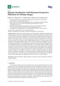
The concept of 3-view rectification using homographies is illustrated in Figure 3. The triplet is processed pair by pair therefore producing 4 homographies. The images are denoted 1,2 and 3. For 1 and 2, the rectification without the distortion reduction step gives us H1 and H2 . Similarly, for images 2 and 3 the rectification without distortion reduction gives us H20 and H3 . The rectification does not include the distortion since we want to stay consistent on the type of images we are working on : they are all affected by the same type of effects. The distortion reduction will therefore be the last phase of this process. We know that, by definition, a rectified configuration that sends all epipoles to infinity (i.e. where all epipolar lines are parallel) is one where all the image planes are coplanar. The solution we are seeking is then based on an attempt to find a common plane on which lie all rectified images. Homographies are projective linear transformations that can be chained in order to project an image plane over a new plane. We therefore want to build a homography-based solution that relies on composing the plane transformations that will bring all images of the triplet onto a common plane as illustrated in Fig.3.
11
(a) Original vertical pair
(b) Rectified vertical pair
Figure 2: Rectification for a “vertical” stereo pair.
12
Figure 3: Rectification principle for a triplet of images.
4.1
Horizontal triplets
The middle image 2 is common to the two pairs so we have H2 and H20 . Each of the computed homographies ’sends’ the image plane 2 on two different planes containing respectively the rectified image 1 i.e P12 and the rectified image 3 i.e P23 (see Figure 3). Our goal here is to find a way to transfer the plane P23 to P12 ; as a matter of fact we want to find the homography h between these two planes. This is done as follows: • Image 2 is transferred to plane P12 with H2 • Image 2 is transferred to plane P23 with H20 • Image 3 is transferred to plane P23 with H3 • h between P12 and P23 is therefore given by h = H2 H20−1 : this is the “unification” mentioned earlier. Using the projection of the middle image in two different planes to deduct the relationship between both involved planes. 13
• Image 3 can therefore be transferred to plane P12 by transiting through P23 using H30 given by : H30 = hH3 = H2 H20 −1 H3
(13)
These steps essentially evaluate the homography H30 that sends the rectified version of image 3 to the plane containing the already rectified versions on image 1 and 2 by using the redundant data provided by the middle image. Finally, distortion reduction for the horizontal configuration is applied to each homography H1 , H2 and H30 to insure that the y coordinates are left untouched.
4.2
“L-triplets”
The case of ’L’-shaped triplets is a combination of a vertical pair and a horizontal pair. All steps in the horizontal triplet procedure are repeated except for what follows: • The pair 1, 2 is rectified using the vertical pair approach without the distortion reduction procedure (Section 3). • The distortion rectification step uses the vertical distortion reduction approach for the rectified images 1 and 2. For image 3, the distortion reduction is also applied with the vertical approach described in section 2.6 to level the images 2 and 3 along the vertical axis.
5
Results and Observations for image triplets
For triplets of images, we have an example of a horizontal rectified triplet in Fig.4 with the original images in Fig.5. A few epipolar lines are drawn across the 3 images to show the consistency in the rectification process. For the sake of comparison, the first example of “L”-shaped triplet is the same as the one processed in [9]. The original triplet is shown in Fig.6. The result obtained in [9] are given in Fig.7. The result obtained using the homographybased approach presented in this paper is given Fig.8. The desired epipolar lines are obtained in both cases. The effect of the distortion reduction is however well noticeable when comparing both results the set in Fig.8 looking less distorted and closer to the original images than the set in Fig.7. 14
Figure 4: Original triplet of images : horizontal configuration.
Figure 5: Rectified triplet of images : horizontal configuration.
Figure 6: Original “L”-triplet (courtesy of C. Sun [9])
15
Figure 7: Results obtained by C. Sun approach (courtesy of C. Sun [9])
Figure 8: Results obtained by homography-based approach
16
Figure 9: Original triplet of images of the second example : L configuration
Fig.9 and Fig.10 show another example of rectified “L”-shaped triplet of images.
5.1
Observations
An important observation mentioned earlier and in [8] is the fact that the rectification is ineffective for images where the epipoles appear in the image plane; suitable images are therefore to be used. This limitation concerning the capture process is however not detrimental to stereo systems that usually use a quasi parallel setup for the image planes. Another observation, that is rather obvious, is that a pair or triplet of images has to be taken close to the ideal configuration before using the corresponding rectification algorithm: i.e. it is impossible to rectify a vertical stereo pair of images with the horizontal stereo rectification approach. Finally an important source of error is clearly the fundamental matrix approximation. For example note that well spread matches over the images help improve radically the fundamental matrix which otherwise ends up being very localized 17
Figure 10: Rectified triplet of images of the second example : L configuration
and valid only for a few points. It is therefore a very important step that should be handled with care and carried out following one of the many existing techniques. For a set of algorithms, we suggest the reader to refer to [12].
6
Conclusion
This paper presented a homography-based approach for the rectification of image triplets. The method has the advantage of being suitable for uncalibrated environments as well as producing rectifying homographies with low distortion effects using solely the fundamental matrix. The approach used a homography composition in order to rectify all images by projecting them on a common plane with the constraint of epipoles at infinity in the destination image plane. This proved to be a simple operation to carry out once the pair-wise rectifications were completed. The cases of horizontal triplets and “L”-shaped triplets were both treated. Results were obtained on different sets of images and these were further visually improved when the proper distortion reduction was applied as the final step. A few observations were made as far as the performance of the basic stereo algo18
rithm is concerned and the influence of matches and the fundamental matrix on the overall process.
References [1] L. An, Y. Jia, J. Wang, X. Zhang, and M. Li. An efficient rectification method for trinocular stereovision. In Int. Conf. on Pattern recognition, pages IV: 56–59, 2004. [2] N. Ayache and F. Lustman. Trinocular stereo vision for robotics. IEEE Trans. Pattern Anal. Mach. Intell., 13(1):73–85, 1991. [3] R. Hartley. In defense of the 8-point algorithm. IEEE trans. Pattern Analysis and Machine Intelligence, 19:580–593, 1995. [4] R. Hartley. Theory and practice of projective rectification. Int. Journal Computer Vision, 35(2):115–127, 1999. [5] R. I. Hartley and A. Zisserman. Multiple View Geometry in Computer Vision. Cambridge University Press, ISBN: 0521540518, second edition, 2004. [6] C. Loop and Z. Zhang. Computing rectifying homographies for stereo vision. In in Proc. IEEE Conf. on Computer Vision and Pattern Recognition, pages 125–131, 1999. [7] D. G. Lowe. Distinctive image features from scale-invariant keypoints. Int. J. Comput. Vision, 60(2):91–110, 2004. [8] J. Mallon and P. Whelan. Projective rectification from the fundamental matrix. Image and Vision Computing, 23(7):643–650, July 2005. [9] C. Sun. Uncalibrated three-view image rectification. Image and Vision Computing, 21(3):259–269, 2003. [10] A. Whitehead and G. Roth. The projective vision toolkit. In Proceedings, Modelling and Simulation., pages 204–209, 2000. [11] H. Zhang, J. Cech, R. Sara, F. Wu, and Z. Hu. A linear trinocular rectification method for accurate stereoscopic matching. In British Machine Vision Conf., pages 281–290, 2003. [12] Z. Zhang. Determining the epipolar geometry and its uncertainty: A review. Technical Report 2927, Sophia-Antipolis Cedex, France, 1996. [13] J. Zhou and B. Li. Image rectification for stereoscopic visualization. J. Opt. Soc. Am. A, 25:2721–2733, November 2008.
19