1Department of Computer Science and Engineering, Lehigh University, Bethlehem, PA 18015. 2Computational Biomedicine Imaging and Modeling Center, ...
Active Volume Models with Probabilistic Object Boundary Prediction Module Tian Shen1 , Yaoyao Zhu1 , Xiaolei Huang1 , Junzhou Huang2 , Dimitris Metaxas2 , and Leon Axel3 1
Department of Computer Science and Engineering, Lehigh University, Bethlehem, PA 18015 2 Computational Biomedicine Imaging and Modeling Center, Rutgers University, NJ 08854 3 Department of Radiology, New York University School of Medicine, New York, NY 10016 Abstract. We propose a novel Active Volume Model (AVM) which deforms in a free-form manner to minimize energy. Unlike Snakes and level-set active contours which only consider curves or surfaces, the AVM is a deforming object model that has both boundary and an interior area. When applied to object segmentation and tracking, the model alternates between two basic operations: deform according to current object prediction, and predict according to current appearance statistics of the model. The probabilistic object prediction module relies on the Bayesian Decision Rule to separate foreground (i.e. object represented by the model) and background. Optimization of the model is a natural extension of the Snakes model so that region information becomes part of the external forces. The AVM thus has the efficiency of Snakes while having adaptive region-based constraints. Segmentation results, validation, and comparison with GVF Snakes and level set methods are presented for experiments on noisy 2D/3D medical images.
1
Introduction
Boundary extraction is an important task in medical image analysis. The main challenge is to retrieve high-level information from low-level image signals while minimizing the effect of noise, intensity inhomogeneity, and other factors. Model-based methods have been widely used with considerable success. Most noticeable are two types of models: deformable models [1, 2], and statistical shape and appearance model [3, 4]. Kass et al. proposed Snakes [1], which are energy-minimizing splines with smoothness constraints and influenced by image forces. Other parametric models were proposed to incorporate overall shape model constraints [5] and to increase the attraction range of the original Snakes by Gradient Vector Flow (GVF) [6]. Depending solely on image gradient information, however, these methods may be trapped by noise and spurious edges. Region analysis strategies [7, 8] have been incorporated in Snake-like models to improve their robustness to noise. Another class of deformable models commonly used in medical image analysis is level set based geometric models [2]. This approach represents curves and surfaces implicitly as the level set of a higher-dimensional scalar function and the evolution of these implicit models is based on the theory of curve evolution, with speed function specifically designed to incorporate image gradient information. The integration of region information in geometric models has been mostly based on solving the frame partition problem as in Geodesic Active Region [9] and Active contours without edges [10]. In noisy medical images, statistical modeling approaches are adopted by adding some constrains from prior offline learning. Cootes et al. proposed methods for building active shape models [4] and active appearance models [3], by learning patterns of variability from a training set of annotated images. Integrating high-level knowledge, these models deform in ways constrained by the training data. Thus they are often more robust in image interpretation. Image interpretation by shape-appearance joint prior models can be based on image search [4], or by maximizing posterior likelihood of the model given image information, in a Bayesian framework [11]. Shape priors particularly have been
introduced to level-set based cardiac segmentation [12], and to deformable models for constrained segmentation of bladder and prostate [13]. In this paper, we propose an Active Volume Model (AVM) which deforms with constraints from both Region Of Interest (ROI) and image gradient information. The ROI, which represents the predicted object, is obtained from a classification of image features based on model-interior statistics. An approximation of the object appearance statistics, the model-interior statistics are learned adaptively during model evolution. An advantage of the AVM model is that its formulation allows the ROI information to naturally become part of the Snakes external forces; in this way, rapid model deformations can be derived by finding the solution of the Euler equations in a variational framework [1]. In our experimental evaluation on various noisy medical images in 2D/3D, we found that AVM achieved comparable speed with the original Snakes and GVF [6] but with much better robustness and accuracy. The probabilistic ROI boundary-prediction module provides a meaningful classification, in comparison with the thresholding technique in [8]. With similar model initialization, AVM converges much faster (typically within 30 ∼ 40 iterations) than Active contours without edges (ACWE) [10]. While AVM produces a single smooth object boundary surface, the segmentation by ACWE often contains small holes and islands.
2
Methodology
An active volume model is a deforming solid that minimizes internal and external energy. The internal constraint ensures the model has smooth boundary. The external constraints come from image data, priors, and/or user-defined features. Representing the model boundary parametrically, v(s) = (x(s), y(s)), the internal energy term of AVM is defined similar to Active Contour Models. Z 1 (α(s)|vs (s)|2 + β(s)|vss (s)|2 )ds (1) Eint = 0
The external energy function consists of two terms: the gradient term Eg and the region term ER . So the overall energy function is: E = Eint + Eext = Eint + k · (Eg + kext · ER )
(2)
where k is a constant that balances the internal and external forces. kext is a constant that balances the contributions of the gradient term and the region term. Gradient Data Term. The gradient data term can be defined using the gradient map, edge distance map, or a combination of both. Denote a gradient magnitude map or the distance transform of an edge map as Fg , the gradient data term is defined as: Eg =
Z
1
Fg (v(s))ds
(3)
0
Fg =
�
2 Dedge , edge distance map; or 2 − |∇I| , gradient magnitude map
(4)
where Dedge refers to the unsigned distance transform of the edge map, and ∇I represents the image gradient. Region Data Term. A novel aspect of the active volume model is that it learns the appearance statistics of the object of interest dynamically and the model’s deformation is driven by the predicted object-region boundary. External constraints from various sources can be accounted in the Region Data Term by probabilistic integration. Let us
consider that each constraint corresponds to a probabilistic boundary prediction module, and it generates a confidence-rated probability map to indicate the likelihood of a pixel being: +1 (object class), or -1 (non object class). Suppose we have n independent external constraints, the feature used in the kth constraint is fk , and L(v) denotes the label of a pixel v, our approach to combining the multiple independent modules is applying the Bayes rule in order to evaluate the final confidence rate: P r(f1 , f2 , ..., fn |L(v))P r(L(v)) P r(f1 , f2 , ..., fn ) ∝ P r(f1 |L(v))P r(f2 |L(v))...P r(fn |L(v))P r(L(v))
P r(L(v)|f1 , f2 , ..., fn ) =
(5)
For each independent module, the probability P r(fk |L(v)) is estimated based on the active volume model’s interior statistics. Considering a module using intensity statistics, the object region can be predicted according to the current model-interior intensity distribution. For instance, for a pixel v with intensity feature value I(v) = i where i ranges from 0 to 255, we have: P r(i|I) = P r(i, object|I) + P r(i, non object|I) = P r(i|object, I)P r(object|I) + P r(i|non object, I)P r(non object|I)
(6)
In the equation, the intensity distribution over the entire image I, P r(i|I) is known, and we estimate the object-interior distribution P r(i|object, I) by the current model-interior intensity distribution. Therefore, the background distribution can be derived: P r(i|I) − P r(i|object, I)P r(object|I) P r(non object|I)
P r(i|non object, I) =
(7)
Assuming a uniform prior, P r(object|I) = P r(L(v) = object) = 0.5 and P r(non object|I) = P r(L(v) = non object) = 0.5, in Eqn. 7, we are able to compute the background probability P r(i|non object, I). Applying the Bayesian Decision rule, we can obtain a binary map PB that represents the predicted object region; that is, PB (v) = 1 if P r(i|object, I) ≥ P r(i|non object, I), and PB (v) = 0 otherwise. We then apply a connected component analysis algorithm on PB to retrieve the connected component that overlaps the current model. This connected region is considered as the current ROI. Due to noise, there might be small holes that need to be filled before extracting the shape of the ROI, R. (We will discuss how to detect and handle actual holes in the object in Section 2.3). Let us denote the signed distance transform of the current model’s shape as ΦM , and the signed distance transform of the ROI shape as ΦR , the region-based external energy term is defined as: ER =
Z
1
ΦM (v(s))ΦR (v(s))ds
(8)
0
The multiplicative term provides two-way balloon forces that deform the model toward the predicted ROI boundary. This allows flexible model initializations either overlapping the object or inside the object. Some example results are demonstrated in Fig. 3. As one can see in Figure 1(C), the ROI evolves according to the changing object appearance statistics (estimated by model-interior statistics). And the image forces generated by the region term deform the model to converge to the object boundary. The Bayesian-Decision based ROI boundary prediction method outperforms other simple thresholding-on-the-probability-map techniques. For instance, we show the binary map PB generated by applying a threshold of the mean of the model-interior probability in Figure 1(5) for comparison purposes; the ROIs and the converged model result significantly under-estimate the true object volume.
(A)
(B)
(C) (1)
(2)
(3)
(4)
(5)
Fig. 1. Left Ventricle segmentation using AVM. (A) The model on the original image. (B) The binary map PB estimated by intensity-based likelihood maps and applying the Bayesian Decision rule. (C) Distance transform of the ROI boundary. (1) Initial model. (2)-(3) The model after 8 and 18 iterations respectively. (4) Final result after 26 iterations. (5) Converged result using the mean model-interior probability as the threshold.
2.1
Model Dynamic Deformation
Summarizing all terms, the overall energy function is: E=
Z
1
(Eint (v(s)) + k · (Fg (v(s)) + kext · (ΦM (v(s))ΦR (v(s))))) ds
(9)
0
The minimization of E can be achieved by finding the solution of the Euler Equations: Ax + ∂Eext (x, y)/∂x = 0
(10)
Ay + ∂Eext (x, y)/∂y = 0
(11)
where A is the pentadiagonal banded matrix that specifies the internal smoothness constraints of the model [1]. And the model points at iteration t are calculated from model points at iteration t − 1 as follows: xt = (A + γI)−1 (γxt−1 − ∂Eext (xt−1 , yt−1 )/∂x)
(12)
yt = (A + γI)−1 (γyt−1 − ∂Eext (xt−1 , yt−1 )/∂y)
(13)
where matrix I is the identity matrix and γ is the step size. Using the above optimization method, we adopt the following steps to deform the active volume model toward desired object boundary. 1. Initialize the active volume model, smoothness matrix A, step size γ, and calculate the gradient magnitude or edge map. 2. Compute ΦM based on the current model; predict R by applying the Bayesian Decision rule to binarizing the estimated object probability map, and compute ΦR . 3. Deform the model according to Eqns. 12 and 13. 4. Reparameterize the model by resampling along model-boundary curve length, and update the smoothness matrix A. 5. Repeat steps 2-4 until convergence.
2.2 Pseudo-3D Reconstruction Parametric models often encounter efficiency and modeling issues in 3D because of the difficulties in 3D mesh update and reparameterization. Since most 3D volumetric medical images consist of stacks of 2D slices, we adopt an efficient and practical pseudo-3D reconstruction method, which is applicable in a variety of 3D segmentation problems. The basic idea is to perform 2D segmentation in one slice, and then propagate the contour to initialize models in neighboring slices (e.g. above and below). A previous slice’s converged result is used to initialize a new AVM on the current slice and the model then deforms till convergence. To construct a 3D mesh model from the stack of 2D contours, we apply a shape registration algorithm using the implicit distancetransform representation [14] on pair-wise contours. Fifty sample points are taken from the first contour model, and correspondences for these points are computed sequentially on all other contours by shape registration. Once the segmentation is complete in 3D and correspondences between the stack of 2D contours are established, the 3D result is rendered as a triangle mesh in OpenGL. Interactive editing of the segmentation can be performed on individual 2D slices, and after editing, correspondences need to be recomputed only for the slices immediately adjacent to the edited slice. Figure 2 shows an example pseudo-3D reconstruction result of the left ventricle using a heart CT volume.
(a)
(b)
(c)
(d)
(e)
Fig. 2. Pseudo-3D segmentation and reconstruction. (a) Illustrating the “stack of contours” concept. (b)-(c) left ventricle (LV) and aorta showing segmentation on individual slices; LV is based on 82 slices and aorta 50 slices. (d)-(e) Complete reconstruction result with aorta, left atrium (LA) and LV. The aorta consists of 136 slices, LA consists of 101 and LV of 146 slices.
2.3 Detecting Change of Topology We explicitly model topology changes by detecting holes in the volumetric model. Different from level set methods, our explicit hole-detection step has stricter requirement so that the only pixels considered belonging to a hole inside the AVM are those that are consistently classified to the background class for a number of iterations and connect to cover a relatively large fraction (≥ 10%) of the model volume. It should be noted that we always exclude pixels that are classified to background inside the AVM when updating object statistics. If a hole is detected, a new model spawns off to represent the hole structure. The original model is now a compound object with geometry defined by Constructive Solid Geometry (CSG). Interior of the hole is excluded from computing the compound model statistics and the new hole model evolves and deforms on its own without affecting the compound model.
3
Experimental Results
We have experimented with the active volume model for extracting boundaries in various medical images. For images with no clear edges, such as ultrasound images, a smaller step size γ is required. For MRI or CT images, we use a larger step size. We first test the model by using a set of cardiac CT images. Considering that the CT images give relatively reliable edges and gradients, we select a large step size. On a CT image with a stack of 303 2D slices, the model converges within 15 iterations for every slice (see Figure 3). Figure 3(A) also shows that model initialization can either partially
(A)
(B) (1)
(2)
(3)
(4)
(5)
Fig. 3. Cardiac CT images. (A) Initial model. (B) Final converged result after (1)7 (2)8 (3)5 (4)6 (5)14 iterations.
overlap the object or be completely inside the object. The model is able to expand or shrink to converge to the boundary of the object that dominates the model appearance. We also test the model on a variety of CTA and MRI medical images. Figure 4 shows example segmentation results. When segmenting vessel boundaries in CTA images (Figure 4(4) & (5)), we chose a greater coefficient k in Eqn. 9 to avoid the model shrinking to a dot, since the object covers a very small region in the image. For all the images shown in Figure 4, we present comparison between the proposed active volume model (AVM), the Gradient Vector Flow (GVF) model [6], and the level-set based Active Contours without Edges (ACWE) [10]. The GVF implementation is from the original authors (http://iacl.ece.jhu.edu/projects/gvf/snakedemo/) and the ACWE implementation is by Michael Wasilewski (http://www.postulate.org/segmentation.php); we kept the default parameter settings in their original code. The parameters in AVM and the two compared methods are listed in Table 3. The efficiency of AVM is comparable to the original Snakes and to GVF, while the AVM’s accuracy is better. AVM runs much faster than ACWE. AVM produces a smooth boundary directly while the ACWE result contains small holes and islands. Table 3 summarizes the comparison in efficiency, and Figure 4(C)&(D) demonstrate the GVF and ACWE results, in comparison with the AVM result in Figure 4(B). k kext 30.0 30.0 α β γ κ µ σ Gradient vector flow 0.05 0.0 1.0 0.6 0.1 5.0 λ λ ǫ µ ν Active contours without edges 1 2 1.0 1.0 1.0 506.25 0.0 Table 1. Parameters used in implementations when comparing AVM, GVF, and ACWE methods in Figure 4. Active volume model
Model Active volume model Gradient vector flow
Case 1 2 3 4 Iteration number 10 26 31 8 Iteration number 80 40 30 70 Running time(seconds) 253.5 185.8 15.1 16.5 Active contours without edges Iteration number 1600 800 200 100 Table 2. Running time and number of iterations for Figure 4.
5 9 15 12.9 100
We use a set of ultrasound images to test the robustness of the model to noise. Since there is no clear contrast edges in ultrasound images to certify the object boundary, the region-based properties of AVM become very important. Figure 5 shows segmentation results for ultrasound images, in which there are noisy gradients and spurious edges inside the ROI. In this case, the object prediction represented by the ROI is the only reliable information that enabled the finding of object boundary.
(A)
(B)
(C)
(D) (1)
(2)
(3)
(4)
(5)
Fig. 4. Segmentation result for MRI and CTA images. (A) Initial model. (B) Final coverged result after (1)10 (2)26 (3)31 (4)8 (5)9 iterations. (C) Results from GVF after (1)80 (2)40 (3)30 (4)70 (5)15 iterations. (D) Results from Active contours without edges after (1)1600 (2)800 (3)200 (4)100 (5)100 iterations.
Finally, we test the running time and perform validation of the pseudo-3D reconstruction. On a workstation with Intel processor Xeon 5160, the processing time for segmentation and reconstruction shown in Figure 2(a) is 62 seconds, and the time for Figure 2(b) is 26 seconds. Therefore the active volume model is fast enough to be used in near real-time 3D reconstruction. Segmentation accuracy is also validated by comparing to gold standard generated by an expert using methods described in [15]. We performed validation on the 3D left ventricle reconstruction based on 82 slices (Figure 2(a)). The mean values of sensitivity and specificity are 95.7% and 99.7%, respectively. The mean value of the Dice similarity coefficient (DSC) is 97.6%.
4
Discussion
In this paper, we proposed a novel active volume model, which is a natural extension of parametric deformable models to integrate object appearance and region information. The main contributions include: (1) a clean formulation to integrate online learning and adaptive region statistics into active contours, (2) an efficient optimization framework that enables very fast gradient- and appearance-statistics based model deformations, and (3) the combination of multiple sources of information in a unified framework for object region and boundary prediction. Using various experiments on medical images, we demonstrated that our model can perform segmentation efficiently and reliably on CT, CTA, MRI and ultrasound images. In the future, we plan to experiment with true 3D active volume models so that data in the 3D evolving model can be incorporated into the ROI estimation. We will also integrate texture statistics and offline-learned prior models in the framework. Acknowledgments. We would like to thank Dr. Yong Zhang and Dr. Stephen Wong for providing the CTA images, Dr. Chenyang Xu for the heart and brain MRI images,
(A)
(B) (1)
(2)
(3)
(4)
Fig. 5. Segmentation result for ultrasound images. (A) Initial model. (B) Final converged result after (1)21 (2)27 (3)35 (4)23 iterations.
and Dr. Kaisar S. Alam for the ultrasound images. This work is supported by a research award to Dr. Xiaolei Huang from the Christian R. and Mary F. Lindback Foundation.
References 1. Kass, M., Witkin, A., Terzopoulos, D.: Snakes: Active contour models. Int’l Journal on Computer Vision 1 (1987) 321–331 2. Malladi, R., Sethian, J., Vemuri, B.: Shape modeling with front propagation: A level set approach. IEEE Trans. on Pattern Analysis and Machine Intelligence 17(2) (1995) 158–175 3. Cootes, T., Edwards, G., Taylar, C.: Active appearance models. Proc. Of European Conf. on Computer Vision 2 (1998) 484–498 4. Cootes, T., Taylor, C., Cooper, D., Graham, J.: Active shape model - their training and application. Computer Vision and Image Understanding 61 (1995) 38–59 5. Staib, L., Duncan, J.: Boundary finding with parametrically deformable models. IEEE Trans. on Pattern Analysis and Machine Intelligence 14(11) (1992) 1061–1075 6. Xu, C., Prince, J.: Snakes, shapes and gradient vector flow. IEEE Trans. on Image Processing 7 (1998) 359–369 7. Zhu, S., Yuille, A.: Region Competition: Unifying snakes, region growing, and Bayes/MDL for multi-band image segmentation. IEEE Trans. on Pattern Analysis and Machine Intelligence 18(9) (1996) 884–900 8. Huang, X., Metaxas, D., Chen, T.: Metamorphs: Deformable shape and texture models. In: Proc. of IEEE Computer Society Conf. on Computer Vision and Pattern Recognition. 496–503 9. Paragios, N., Deriche, R.: Geodesic active regions and level set methods for supervised texture segmentation. The International Journal of Computer Vision 46(3) (2002) 223–247 10. Chan, T., Vese, L.: Active contours without edges. IEEE Trans. on Image Processing 10 (2001) 266–277 11. Yang, J., Duncan, J.: 3d image segmentation of deformable objects with joint shape-intensity prior models using level sets. Medical Image Analysis 8(3) (September 2004) 285–294 12. Kohlberger, T., Cremers, D., Rousson, M., Ramaraj, R., Funka-Lea, G.: 4d shape priors for a level set segmentation of the left myocardium in spect sequences. In: MICCAI (1). (2006) 92–100 13. Costa, M., Delingette, H., Novellas, S., Ayache, N.: Automatic segmentation of bladder and prostate using coupled 3d deformable models. In: MICCAI (1). (2007) 252–260 14. Huang, X., Paragios, N., Metaxas, D.: Shape registration in implicit spaces using information theory and free form deformations. IEEE Trans. on Patt. Anal. & Mach. Intell. 28(8) (2006) 1303–1318 15. Popovic, A., de la Fuente, M., Engelhardt, M., Radermacher, K.: Statistical validation metric for accuracy assessment in medical image segmentation. International Journal of Computer Assisted Radiology and Surgery (2007) 169–181