Intelligent Systems under grant # 0546467 and the Air Force. Office of Scientific Research under STTR Contract FA9550-. 06-C-0088. Nicholas Roy and Daniela ...
Probabilistic Models of Object Geometry for Grasp Planning Jared Glover, Daniela Rus and Nicholas Roy Computer Science and Artificial Intelligence Laboratory Massachusetts Institute Of Technology Cambridge, MA 02139 {jglov,rus,nickroy}@mit.edu Abstract— Robot manipulators generally rely on complete knowledge of object geometry in order to plan motions and compute successful grasps. However, manipulating real-world objects poses a substantial modelling challenge. New instances of known object classes may vary from learned models. Objects that are not perfectly rigid may appear in new configurations that do not match any of the known geometries. In this paper we describe an algorithm for learning generative probabilistic models of object geometry for the purposes of manipulation; these models capture both non-rigid deformations of known objects and variability of objects within a known class. Given a single image of partially occluded objects, the model can be used to recognize objects based on the visible portion of each object contour, and then estimate the complete geometry of the object to allow grasp planning. We provide two main contributions: a probabilistic model of shape geometry and a graphical model for performing correspondence between shape descriptions. We show examples of learned models from image data and demonstrate how the learned models can be used by a manipulation planner to grasp objects in cluttered visual scenes.
I. I NTRODUCTION Robot manipulators largely rely on complete knowledge of object geometry in order to plan their motion and compute successful grasps. If an object is fully in view, the object geometry can be inferred from sensor data and a grasp computed directly. If the object is occluded by other entities in the scene, manipulations based on the visible part of the object may fail; to compensate, object recognition is often used to identify the location of the object and compute the grasp from a prior model. However, new instances of a known class of objects may vary from the prior model, and known objects may appear in novel configurations if they are not perfectly rigid. As a result, manipulation can pose a substantial modelling challenge when objects are not fully in view. Consider the camera image1 of four toys in a box in figure 1(a). Having a prior model of the objects is extremely useful in that visible segments (such as the three visible parts of the stuffed bear) can be aggregated into a single object, and a grasp can be planned appropriately as in figure 1(b). However, having a prior model of the geometry of every object in the world is not only infeasible but unnecessary. Although an object such as the stuffed bear may change shape as it is handled and placed in different configurations, the 1 Note that for the purposes of reproduction, the images have been cropped and modified from the original in brightness and contrast. They are otherwise unchanged.
(a) Original Image
(b) Recovered Geometries
Figure 1. (a) A collection of toys in a box. The toys partially occlude each other, making object identification and grasp planning difficult. (b) By using learned models of the bear, we can identify the bear from the three visible segments and predict its complete geometry (shown by the red line; the dashed lines are the predicted outline of the hidden shape). This prediction of the complete shape can then be used in planning a grasp of the bear (planned grasp points shown by the blue circles).
general shape in terms of a head, limbs, etc. are roughly constant. Regardless of configuration, a single robust model which accounts for deformations in shape should be sufficient for recognition and grasp planning for most object types. In this paper we describe an algorithm for learning a probabilistic model of visual object geometry. Although statistical models of shape geometry have received attention in a number of domains including computer vision [9, 7] and robotics, existing techniques have largely been coupled to tasks such as shape localization [7], recognition and retrieval [18, 1]. Many effective recognition and retrieval algorithms are discriminative in nature and create representations of the shape that make it difficult to perform additional inference such as recovering hidden object geometry. Our primary contribution is an algorithm for learning generative models of object shapes as dense 2-D contours, as we are specifically interested in object geometry for manipulation planning. We use a model of object shape, known as Procrustean shape [6, 13], that provides model invariance to translation, scale and rotation; we generalize this technique to learn object models that are robust to object variation and deformations. One of the challenges in inferring dense models of shape is that in order to compute the likelihood of a particular shape given a model, we must a priori know which points in the measured shape correspond to which points in the model. Thus, our second contribution is to provide a graphical model for computing correspondences between shapes as a pre-processing step to the model learning. We conclude with experimental demonstrations of object detection in cluttered
Algorithm 1 The Manipulation Process. Require: An image of a scene, and learned models of objects 1: Segment the image into object components 2: Extract contours of components 3: Determine maximum-likelihood correspondence between observed contours and known models 4: Infer complete geometry of each object from matched contours 5: Return planned grasp strategy based on inferred geometries
(a) Example Object
(b) Class Distribution
Figure 2. (a) An example image of a chalk compass. The compass can deform by opening and closing. (b) Sample shapes from the learned distribution along different eigenvalues of the distribution.
scenes, geometry prediction and grasp planning. II. T HE M ANIPULATION P ROCESS Our goal is to manipulate an object in a cluttered scene– for example to grasp the bear in figure 1(a). Our proposed manipulation process is given in algorithm 1. The input to the algorithm is a single image which is first segmented into perceptually similar regions. (Although image segmentation is a challenging research problem, it is outside the scope of this paper and we rely on existing segmentation algorithms such as [23].) The boundaries or contours of the image segments are extracted, and it is these representations of object geometry that we use throughout this paper. We first describe how to learn a generative probabilistic model of a class of objects, given a set of object contours of the same class. Using the learned models of class geometry, we next describe how different instances of an object class can be recognized and localized in a single image of partially occluded objects. We use the generative model to infer the hidden parts of each object in order to complete the model of each object. Finally, we describe how the inferred complete geometry can be used to compute a grasp. III. P ROBABILISTIC M ODELS OF 2-D S HAPE Formally, we represent an object Z in an image as a set of n ordered points on the contour of the shape, {z1 , z2 , . . . zn }, in a two-dimensional Euclidean space, so that zi = (xi , yi )). Our goal is to learn a probabilistic, generative model of Z. We begin by making the contour invariant with respect to position and scale, normalizing Z so as to have unit length with centroid at the origin, that is, Z′ τ
= {z′ i = (xi − x ¯, yi − y¯)} Z′ = , |Z′ |
(1) (2)
where τ is the pre-shape of the contour Z. Since τ is a unit vector, the space of all possible pre-shapes of n points is the unit hyper-sphere, S2n−3 , called pre-shape space. Since we ∗ can rotate any pre-shape through a great circle orbit O(τ ) of maximal length of the hypersphere without changing the geometry of z, we define the “shape” of Z as an equivalence class of pre-shapes over rotations. If we can define a distance metric between shapes, then we can infer a parametric distribution over the shape space. The spherical geometry of the pre-shape space requires a geodesic distance rather than Euclidean distance. The distance between
τ1 and τ2 is defined as the smallest distance between their orbits, dp [τ1 , τ2 ] d(ϕ, ψ)
= inf[d(ϕ, ψ) : ϕ ∈ O(τ1 ), ψ ∈ O(τ2 )] (3) = cos−1 (ϕ · ψ). (4)
Kendall [13] defined dp as the Procrustean metric where d(ϕ, ψ) is the geodesic distance between ϕ and ψ. We can solve for the minimization of equation (3) in closed form by representing the points of τ1 and τ2 in complex coordinates, which naturally encode rotation in the plane by scalar complex multiplication. This gives dp as cos−1 |τ2H τ1 |
dp [τ1 , τ2 ] =
(5)
τ2H
is the Hermetian, or complex conjugate transpose where of the complex vector τ2 . A. Learning Shape Models In order to complete our probabilistic model of object geometry, we compute a distribution for each object class from training images. We choose a Gaussian approximation to the distribution over shapes, which only requires us to compute the mean and covariance of the training data. This Gaussian lies in the tangent space to the hypersphere at the mean shape vector. For each object class i, we compute a mean shape µi , from a set of pre-shapes {τ1 , . . . , τn } by minimizing the sum of Procrustean distances from each pre-shape to the mean, X µi = arginf [dp (τj , µ)]2 , (6) µ
j
subject to the constraint that kµi k = 1. In two dimensions, this minimization can be done in closed form; iterative algorithms exist for computing µi in higher dimensions [2, 10]. In order to estimate the covariance of the shape distribution from the sample pre-shapes {τ1 , . . . , τn }, we rotate each τj to fit the mean shape µi (i.e. to minimize Procrustean distance), and then project the rotated pre-shapes into the tangent space of the pre-shape hypersphere at the mean shape. We then use Principle Components Analysis (PCA) in tangent space to model the principle axes of the Gaussian shape distribution of {τ1 , . . . , τn }. Figure 2(a) shows one example out of a training set of images of a deformable object. Figure 2(b) shows sample objects drawn from the learned distribution. The red contour is the mean, and the green and blue samples are taken along the first two principal components of the distribution.
Figure 3. Order-preserving matching (left) vs. Non-order-preserving matching (right). The thin black lines depict the correspondences between points in the red and blue contour. Notice the violation of the cyclic-ordering constraint between the right arms of the two contours in the right image.
B. Shape Classification Given k previously learned shape classes C1 , . . . , Ck with shape means µ1 , . . . , µk and covariance matrices Σ1 , . . . , Σk , and given a measurement m of an unknown object shape, we can now compute the likelihood of a shape class given a measured object: {P (Ci |m) : i = 1 . . . k}. The shape classification problem is to find the maximum likelihood class, ˆ which we can compute as C, Cˆ = arg max P (Ci |m) Ci
= arg max P (m|Ci )P (Ci ). Ci
(7) (8)
Given the mean and covariance of a shape class, we can compute the likelihood of a measured object given a class as p(m|Ci ) = N (m; µi , Σi ). Assuming a uniform prior on Ci , we can compute the maximum likelihood class as Cˆ = argmax N (m; µi , Σi ).
(9)
Ci
IV. DATA A SSOCIATION AND S HAPE C ORRESPONDENCES Evaluating the likelihood given by equation 9 requires calculating the Procrustes distance dp between the observed contour m and the mean µi . The distance between any two contours τ1 and τ2 implicitly assumes that there is a known correspondence between a point xi in τ1 and some point yj in τ2 . (There is also an assumption that the lengths of τ1 and τ2 are the same.) Before we can compute the probability of a contour, or even learn the mean and covariance of a set of pre-shapes, we must therefore be able to compute the correspondences between contours, matching each point in τ1 to a corresponding point on τ2 . Solving for the most likely correspondences between sets of data is an open problem in a number of fields, including computer vision and robot mapping. As object geometries vary due to projection distortions, sensor error, or even natural object dynamics, determining which part of an object image corresponds to which part of a previous image is non-trivial. Furthermore, by the nature of object contours, our specific shape correspondence problem contains a cyclic orderpreserving constraint, that is, correspondences between the two contours cannot “cross” each other. Scott and Nowak [22] define the Cyclic Order-Preserving Assignment Problem (COPAP) as the problem of finding an optimal one-to-one matching such that the assignment of corresponding points preserves
the cyclic ordering inherited from the contours. Figure 3 shows an example set of correspondences (the thin black lines) that preserve the cyclic order-preserving constraint on the left, whereas the correspondences on the right of figure 3 violate the constraint at the right of the shape (notice that the association lines cross.) In the following sections, we show how the original COPAP algorithm can be written as a linear graphical model with the introduction of additional book-keeping variables. Our goal is to match the points of one contour, x1 , . . . , xn to the points on another, y1 , . . . , ym . Let Φ denote a correspondence vector, where φi is the index of y to which xi corresponds; that is: xi → yφi . We wish to find the most likely Φ given x and y, that is, Φ∗ = argmaxΦ p(Φ|x, y). If we assume that the likelihood of individual points {xi } and {yj } are conditionally independent given Φ, then Φ∗
= =
1 p(x, y|Φ)p(Φ) Z Φ n 1 Y argmax p(xi , yφi )p(Φ) Z i=1 Φ
argmax
(10) (11)
where Z is a normalizing constant.
A. Priors over Correspondences There are two main terms to equation (10), the prior over correspondences, p(Φ), and the likelihood of object points given the correspondences, p(xi , yφi ). We model the prior over correspondences, p(Φ), as an exponential distribution subject to the cyclic-ordering constraint. We encode this constraint in the prior by allowing p(Φ) > 0 if and only if ∃ω s.t. φω < φω+1 < · · · < φn < φ1 < · · · < φω−1 . (12) We call ω the wrapping point of the assignment vector Φ. Each assignment vector, Φ, which obeys the cyclic-ordering constraint must have a unique wrapping point, ω. Due to variations in object geometry, the model must allow for the possibility that some sequence of points of {xi , . . . , xj } do not correspond to any points in y, for example, if sensor noise has introduced spurious points along an object edge or if the shapes vary in some significant way, such as an animal contour with three legs where another has four. We “skip” individual correspondences in x by allowing φi = 0. (Points yj are skipped when ∄i s.t. φi = j). We would like to minimize the number of such skipped assignments, so we give diminishing likelihood to φ as the number of skipped points increases. Therefore, for Φ with k skipped assignments (in x and y), ( 1 exp{−k(Φ) · λ} if Φ is cyclic ordered p(Φ) = ZΦ (13) 0 otherwise, where ZΦ is a normalizing constant and λ is a likelihood penalty for skipped assignments. B. Correspondence Likelihoods Given an expression for the correspondence prior, we also need an expression for the likelihood that two points xi and yφi correspond to each other, p(xi , yφi ), which we model as
the likelihood that the local geometry of the contours match. Section III described a probabilistic model for global geometric similarity using the Procrustes metric, and we specialize this model to computing the likelihood of local geometries, which we call the Procrustean Local Shape Distance (PLSD). We first need a description of the local shape about xi . In order to be robust to the local spacing of x’s points, we sample points evenly spaced about xi . We define the local neighborhood of size k about xi as: ηk (xi ) = hδxi (−2k ∆), ..., δxi (0), ..., δxi (2k ∆)i
(14)
Φ
where δxi (d) returns the point from x’s contour interpolated a distance of d starting from xi and continuing clockwise for d positive or counter-clockwise for d negative. (Also, δxi (0) = xi .) The parameter ∆ determines the step-size between interpolated neighborhood points, and thus the resolution of the local neighborhood shape. We have found that setting ∆ such that the largest neighborhood is 20% of the total shape circumference yields good results on most datasets. The Procrustean Local Shape Distance, dP LS , between two points, xi and yj is the mean Procrustean shape distance over neighborhood sizes k: Z dP LS (xi , yj ) = ξk · dP [ηk (xi ), ηk (yj )] (15) k
with neighborhood size prior ξ. No closed form exists for this integral so we approximate it using a sum over a discrete set of neighborhood sizes.
C. A Graphical Model for Shape Correspondences Although we assume independence between local features xi and yj , the cyclic-ordering constraint leads to dependencies between the assignment variables φi in a non-trivial way—in fact, the sub-graph of Φ is fully connected since each φi must know the values of all the other assignments, φj , in order to determine whether the matching is order-preserving or not. Computing the maximum likelihood Φ is therefore a nontrivial loopy graphical inference problem. We can avoid this problem and break most of these dependencies by introducing variables αi and ω, where αi corresponds to the last non-zero assignment before φi and ω corresponds to the wrapping point from section IV-A. With these additional variables, each φi depends only on the wrapping point, which is stored in ω as well as the last nonzero assignment, αi ; the cyclic ordering-constraint is thus encoded by pco (φi ), such that 1 : if φi > αi or Zco φi < αi and ωi = i or pco (φi ) = (16) φ i =0 0 : otherwise, which gives
Y 1 (exp{−k(Φ) · λ) pco (φi ). p(Φ) = ZΦ i
wrapping point, ω, to each possible value from 1 to n. Given ω = k, the cycle is broken into a linear chain (according to equation 12), which can be solved by dynamic programming. It is this introduction of the αi and ω variables that is the key to the efficient inference procedure by converting the loopy graphical model into a linear chain. In this approach, the point-assignment likelihoods are converted into a cost function C(i, φi ) by taking a log likelihood, and φ is optimized using Y Y Φ∗ = argmax log p(xi , yφi )p(Φ) pco (φi ) (19)
(17)
(18)
If we initially assign the wrapping point ω, the state vector {αi , φi } then yields a cyclic Markov chain. The standard approach to solving this cyclic Markov chain is to try setting the
i
= argmin Φ
X i
i
!
C(i, φi )
+ λ · k(φ)
(20)
s.t. ∀φi pc o(φi ) > 0 where k(Φ) is the number of points skipped in the assignment Φ. Solving for Φ using equation (20) takes O(n2 m) running time; however a bisection strategy exists in the dynamic programming search graph which reduces the complexity to O(nm log n) [22]. V. S HAPE C OMPLETION We now turn to the problem of estimating the complete geometry of an object from an observation of part of its contour. We phrase this as a maximum likelihood estimation problem, estimating the missing points of a shape with respect to the Gaussian tangent space shape distribution. Let us represent a shape as: z = [z1 z2 ]T
(21)
where z1 = m contains the p points of our partial observation of the shape, and z2 contains the n − p unknown points that complete the shape. Given a shape distribution D on n points with mean µ and covariance matrix Σ, and given z1 containing p measurements (p < n) of our shape, our task is to compute the last n − p points which maximize the joint likelihood, PD (z). (We implicitly assume that correspondences from the partial shape z to the model D are known–we later show how to compute partial shape correspondences in order to relax this assumption.) In order for us to transform our completed vector, z = (z1 , z2 )T , into a pre-shape, we must first normalize translation and scale. However, this cannot be done without knowing the last n − p points. Furthermore, the Procrustes minimizing rotation from z’s pre-shape to µ depends on the missing points, so any projection into the tangent space (and corresponding likelihood) will depend in a highly non-linear way on the location of the missing points. We can, however, compute the missing points z2 given an orientation and scale. This leads to an iterative algorithm that holds the orientation and scale fixed, computes z2 and then computes a new orientation and scale given the new z2 . The translation term can then be computed from the completed contour z. We derive z2 given a fixed orientation θ and scale α in the following manner. For a complete contour z, we normalize for orientation and scale using 1 (22) z′ = R θ z α
from which to sample orientations. Similarly, we can sample scales from a Gaussian with mean α0 –the ratio of scales of the partial shapes z1 and µ1 as in α0 =
Figure 4. An example of occluded objects, where the bear occludes the compass. (a) The original image and (b) the image segmented into (unknown) objects. The contour of each segment must be matched against a known model.
where Rθ is the rotation matrix of θ. To center z′ , we then subtract off the centroid: 1 w = z′ − Cz′ (23) n where C is the 2n × 2n checkerboard matrix, 1 0 ··· 1 0 0 1 · · · 0 1 . . . . . ... ... C= (24) .. .. . 1 0 · · · 1 0 0 1 ··· 0 1
kz1 − p1 C1 z1 k kµ1 − p1 C1 µ1 k
.
(30)
Any sampling method for shape completion will have a scale bias–completed shapes with smaller scales project to a point closer to the origin in tangent space, and thus have higher likelihood. One way to fix this problem is to solve for z2 by performing a constrained optimization on dΣ where the scale of the centered, completed shape vector is constrained to have unit length: 1 (31) kx′ − Cx′ k = 1. n This constrained optimization problem can be attacked with the method of Lagrange multipliers, and reduces to the problem of finding the zeros of a (n−p)th order polynomial in one variable, for which numerical techniques are well-known.
Thus w is the centered pre-shape. Now let M be the matrix that projects into the tangent space defined by the Gaussian distribution (µ, Σ): M = I − µµT
(25)
The Mahalanobis distance with respect to D from M w to the origin in the tangent space is: dΣ = (M w)T Σ−1 M w
(a) Partial contour to be completed
(b) Completed as compass
(c) Completed as stuffed animal
(d) Completed as jump rope
(26)
Minimizing dΣ is equivalent to maximizing PD (·), so we ∂d continue by setting ∂zΣ2 equal to zero, and letting 1 1 C1 ) Rθ1 (27) n α 1 1 (28) W2 = M2 (I2 − C2 ) Rθ2 n α where the subscripts “1” and “2” indicate the left and right sub-matrices of M , I, and C that match the dimensions of z1 and z2 . This yields the following system of linear equations which can be solved for the missing data, z2 : W1 = M1 (I1 −
(W1 z1 + W2 z2 )T Σ−1 W2 = 0
(29)
As described above, equation (29) holds for a specific orientation and scale. We can then use the estimate of z2 to re-optimize θ and α and iterate. Alternatively, we can simply sample a number of candidate orientations and scales, complete the shape of each sample, and take the completion with highest likelihood (lowest dΣ ). To design such a sampling algorithm, we must choose a distribution from which to sample orientations and scales. One idea is to match the partial shape, z1 , to the partial mean shape, µ1 , by computing the pre-shapes of z1 and µ1 and finding the Procrustes fitting rotation, θ∗ , from the pre-shape of z1 onto the pre-shape of µ1 . This angle can then be used as a mean for a von Mises distribution (the circular analog of a Gaussian)
Figure 5. Shape completion of the partial contour of the compass in figure 4. Note that the correct completion (b) captures the knob in the top of the compass. The hypothesized completions in (c) and (d) lead to very unlikely shapes.
A. Partial Shape Class Likelihood Let z = {z1 , z2 } be the completed shape, where z1 is the partial shape corresponding to measurement m, and z2 is unknown. The probability of the class given the observed part of the contour z1 is then Z P (Ci , z1 ) ∝ P (Ci , z1 , z2 )dz2 (32) P (Ci |z1 ) = P (z1 ) Rather than marginalize over the hidden data, z2 , we can ˆ2 , the output of approximate this marginal with an estimate z our shape completion algorithm, yielding: ˆ2 |Ci ) P (Ci |z1 ) ≈ η · P (z1 , z
(33)
where η is a normalizing constant (and can be ignored during ˆ2 |Ci ) is the complete shape class classification), and P (z1 , z likelihood of the completed shape.
B. Partial Shape Correspondences In order to calculate the maximum likelihood shape compleˆ2 with respect to a shape model D, we must know which tion z points in D the observed points z1 correspond to. In practice, z1 may contain multiple disconnected contour segments which must be associated with hidden contour segments to form a complete contour–take for example, the two compass handles in figure 5. Before the hidden contours can be inferred between the handles, observable contours must be ordered. We can constrain the connection ordering by noting that the interiors of all the observed object segments must remain on the interior of any completed shape. For most real-world cases, this topological constraint is enough to identify a unique connection ordering; in cases where the ordering of components is still ambiguous, a search process through the orderings can be used to identify the most likely correspondences. Given a specific ordering of observed contour segments, we can adapt our graphical model from section IV to compute the correspondence between an ordered set of partial contour segments and a model mean shape, µ. First, we add a set of hidden, or “wildcard” points connecting the partial contour segments. This forms a complete contour, zc , where some of the points are hidden and some are observed. We then run a modified COPAP algorithm, where the only modification is that all “wildcard” points on zc may be assigned to any of µ’s points with no cost. (We must still pay a penalty of λ for skipping hidden points, however.) In order to identify how large the hidden contour is (and therefore, how many hidden points should be added to connect the observed contour segments), we use the insight that objects of the same type generally have a similar scale. We can therefore use the ratio of the observed object segment areas to the expected full shape area to (inversely) determine the ratio of hidden points to observed points. If no size priors are available, one may also perform multiple completions with varying hidden points ratios, and select the best completion using a generic prior such as the minimum description length (MDL) criterion. Using this partial shape correspondence algorithm, we employ an iterative procedure to complete the hidden parts of an object contour–(1) compute the partial shape correspondences, (2) complete the shape given the partial correspondences, (3) compute the full shape correspondences from the completed shape to the model, (4) re-complete the shape using the new correspondences, and repeat (3) and (4) until convergence. VI. G RASP P LANNING Recall from Section II that our manipulation strategy is a pipelined process–first, we estimate the complete geometric structure of the scene; then, we plan a grasp. But before we can get into the details about how an individual object is grasped, we must first decide which object to grasp. The problem domains which we are primarily interested in–such as the “box-of-toys” world of Figure 1–are domains in which there is a single “desired” object or object type; for example, a teddy bear. Thus, our ultimate goal is to retrieve a specific object or class of object from the scene. Sometimes, the desired object will be at the top of the pile, fully in view. In this case, after
analyzing the image and recognizing the object, we will be able to plan a grasp to retrieve the object, irrespective of the placement of other objects in the scene. However, if the desired object is occluded, before attempting to pick it up, we must determine the probability that the sensed object is actually the desired object, and the probability that a planned grasp on the accessible part of the object will be successful. If either of these probabilities are below a pre-determined threshold, we first remove one or more occluding objects and then re-analyze the scene before planning a grasp of the desired object. We implement the first test as a threshold on the class likelihood of the sensed object, p(Ci |m) > 0.7; the second test is a function of our strategy for grasping a single object, described below. A. Grasping a Single Object We have developed a grasp planning system for our mobile manipulator (shown in figure 6), a two-link arm on a mobile base with an in-house-designed gripper with two opposable fingers. Each finger is a structure capable of edge and surface contact with the object to be grasped.
Figure 6.
Our mobile manipulator with a two link arm and gripper.
The input to the grasp planning system is the object geometry with the partial contours completed as described in Section V. The output of the system is two regions, one for each finger of the gripper, that can provide an equilibrium grasp for the object following the algorithms for stable grasping described in [19]. Intuitively, the fingers are placed on opposing edges so that the forces exerted by the fingers can cancel each other out. Friction is modeled as Coulomb friction with empirically estimated parameters. The grasp planner is implemented as search for a pair of grasping edges that yield maximal regions for the two grasping fingers using the geometric conditions derived by Nguyen [19]. Two edges can be paired if their friction cones are overlapping. Given two edges that can be paired we identify maximal regions for placing the fingers so that we can tolerate maximal uncertainty in the finger placement using Nguyen’s criterion [19]. If the desired object is fully observed, we can use the above grasping algorithm unchanged. If it is partially occluded, we must filter out finger placements which lie on hidden (inferred) portions of the object’s boundary. If, after filtering out infeasible grasps, there is still an accessible grasp of sufficient quality according to Nguyen’s criterion, we can attempt a grasp of the object.
Object ring bat rat bear fish banana dolphin compass totals
VII. R ESULTS
detect > 5% (a) Original image
(b) Segmentation
(c) Contours
Partial 3/8 7/10 9/13 7/7 9/9 1/2 1/3 37/52 71.15% 42/52 80.77%
Complete 15/15 8/10 4/4 7/7 6/6 1/2 5/5 46/49 93.88% 48/49 97.96%
Table I C LASSIFICATION RATES ON TEST SET.
(d) Bat Completion
(e) Rat Completion
(f) Grasp
Figure 7. An example of a very simple planning problem involving three objects. The chalk compass is fully observed, but the stuffed rat and green bat are partially occluded by the compass. After segmentation (b), the image decomposes into five separate segments shown in (c). The learned models of the bat and the rat can be completed (d) and (e), and the complete contour of the stuffed rat is correctly positioned in the image (f). The two blue circles correspond to the planned grasp that results from the computed geometry.
(a) Original image
(b) Segmentation
(c) Contours
(d) Bear Completion
(e) Dolphin Completion
(f) Grasp
Figure 8. A more complex example involving four objects. The blue bat and the yellow banana are fully observed, but the stuffed bear and dolphin are significantly occluded. After segmentation (b), the image decomposes into five separate segments shown in (c). The learned models of the bear and the dolphin can be completed (d) and (e), and the complete contour of the stuffed bear is is correctly positioned in the image (f). The two blue circles correspond to the planned grasp given the geometry.
We built a shape dataset containing 11 shape classes (6 of which are seen in figures 7 and 8). We collected 10 images of each object type, segmented the object contours from the background, and used the correspondence and shape distribution learning algorithms of sections III and IV to build probabilistic shape models for each class, using contours of 100 points each. We reduced the dimensionality of the covariance using Principal Components Analysis (PCA). Reducing the covariance to three principal components led to 100% prediction accuracy of the training set, and 98% crossvalidated (k = 5) prediction accuracy.
In figures 7 and 8 we show the results of two manipulation experiments, where in each case we seek to retrieve a single type of object from a box of toys, and we must locate and grasp this object while using the minimum number of object grasps possible. In both cases, the object we wish to retrieve is occluded by other objects in the scene, and so a naive grasping strategy would first remove the objects on top of the desired object until the full object geometry is observed, and only then would it attempt to retrieve the object. Using the inferred geometry of the occluded object boundaries to classify and plan a grasp for the desired object, we find in both cases that we are able to grasp the object immediately, reducing the number of grasps required from 3 to 1. In addition, we were able to successfully complete and classify the other objects in each scene, even when a substantial portion of their boundaries was occluded. The classification of this test set of 7 object contours (from 6 objects classes) was 100% (note the correct completions in figures 7 and 8 of the occluded objects). For a more thorough evaluation, we repeated the same type of experiment on 20 different piles of toys. In each test, we again sought to retrieve a single type of object from the box of toys, and in some cases, the manipulation algorithm required several grasps in order to successfully retrieve an object, due to either not being able to find the object right away, or because the occluding objects were blocking access to a stable grasp of the desired object. In total, 52 partial and 49 complete contours were classified, 33/35 grasps were successfully executed (with 3 failures due to a hardware malfunction which were discounted). In table I, we show classification rates for each class of object present in the images. Partially-observed shapes were correctly classified 71.15% of the time, while fully-observed shapes were correctly classified 93.88% of the time. Several of the errors were simply a result of ambiguity–when we examine the > 5% detection rates (i.e. the percentage of objects for which the algorithm gave at least 5% likelihood to the correct class), we see an improvement to 80.77% for partial shapes, and 97.96% for full shapes. While a few of the detection errors were from poor or noisy image segmentations, most were from failed correspondences from the observed contour to the correct shape model. The most common reason for these failed correspondences was a lack of local features for the COPAP algorithm to latch onto with the PLSD point assignment cost. These failures would seem to argue for a combination of local
and global match likelihoods in the correspondence algorithm, which is a direction we hope to explore in future work. VIII. R ELATED W ORK Statistical shape modeling began with the work on landmark data by Kendall [13] and Bookstein [4] in the 1980s. In recent years, more complex statistical shape models have arisen, for example, in the active contours literature [3]. We believe ours is one of the first works to perform probabilistic inference of deformable objects from partially occluded views. In terms of shape classification, shape contexts [1] and spin images [12] provide robust frameworks for estimating correspondences between shape features for recognition and modelling problems; our work is very related but our initial experiments with these descriptors motivated our work for a better shape model for partial views of objects. Classical statistical shape models require a large amount of human intervention (e.g. hand-labelled landmarks) in order to learn accurate models of shape [6]; only recently have algorithms emerged that require little human intervention [9, 7]. We also build on classical and recent results on motion planning and grasping, manipulation, uncertainty for modeling in robot manipulation, POMDPs applied to mobile robots, kinematics, and control. The initial formulation of the problem of planning robot motions under uncertainty was the preimage backchaining paper [16]. It was followed up with further analysis and implementation [5, 8], analysis of the mechanics and geometry of grasping [17], and grasping algorithm that guarantees geometrically closure properties [19]. Lavalle and Hutchinson [15] formulated both probabilistic and nondeterministic versions of the planning problem through information space. Our manipulation planner currently does not take advantage of the probabilistic representation of the object, but we plan to extend our work to this domain. More recently, Grupen and Coelho [11] have constructed a system that learns optimal control policies in an information space that is derived from the changes in the observable modes of interaction between the robot and the object it is manipulating. Ng et al. [21] have used statistical inference techniques to learn manipulation strategies directly from monocular images; while these techniques show promise, the focus has been generalizing as much as possible from as simple a data source as possible. It is likely that the most robust manipulation strategies will result from including geometric information such as used by Pollard and Zordan [20]. IX. C ONCLUSIONS In future work, we hope to demonstrate improved performance on recognition tasks by incorporating additional priors into the correspondence and completion models, in order to bias the inference procedure towards smoother, more natural correspondences and completions. The shape classes that we have found to cause the most problems for our model contain multiple articulations and self-occlusions, which suggests that it may be useful to combine a skeleton or parts-based models with our global parametric models in order to achieve robustness to these highly variable shapes.
X. ACKNOWLEDGEMENTS Jared Glover and Nicholas Roy were supported by the National Science Foundation Division of Information and Intelligent Systems under grant # 0546467 and the Air Force Office of Scientific Research under STTR Contract FA955006-C-0088. Nicholas Roy and Daniela Rus were supported by the National Science Foundation Division of Computer and Network Systems under grant # 0707601. Daniela Rus was supported by the National Science Foundation under grants # 0426838 and 0735953, and Boeing. R EFERENCES [1] Serge Belongie, Jitendra Malik, and Jan Puzicha. Shape matching and object recognition using shape contexts. IEEE Trans. Pattern Analysis and Machine Intelligence, 24(24):509–522, April 2002. [2] Jos M. F. Ten Berge. Orthogonal procrustes rotation for two or more matrices. Psychometrika, 42(2):267–276, June 1977. [3] A. Blake and M. Isard. Active Contours. Springer-Verlag, 1998. [4] F.L. Bookstein. A statistical method for biological shape comparisons. Theoretical Biology, 107:475–520, 1984. [5] Bruce Donald. A geometric approach to error detection and recovery for robot motion planning with uncertainty. Artificial Intelligence, 37:223– 271, 1988. [6] I. Dryden and K. Mardia. Statistical Shape Analysis. John Wiley and Sons, 1998. [7] G. Elidan, G. Heitz, and D. Koller. Learning object shape: From drawings to images. In Proceedings of the Conference on Computer Vision and Pattern Recognition (CVPR), 2006. [8] Michael Erdmann. Using backprojection for fine motion planning with uncertainty. IJRR, 5(1):240–271, 1994. [9] P. Felzenszwalb. Representation and detection of deformable shapes. IEEE Trans. Pattern Analysis and Machine Intelligence, 27(2), 2005. [10] J. C. Gower. Generalized procrustes analysis. Psychometrika, 40(1):33– 51, March 1975. [11] Roderic A. Grupen and Jefferson A. Coelho. Acquiring state from control dynamics to learn grasping policies for robot hands. Advanced Robotics, 16(5):427–443, 2002. [12] Andrew Johnson and Martial Hebert. Using spin images for efficient object recognition in cluttered 3-d scenes. IEEE Transactions on Pattern Analysis and Machine Intelligence, 21(5):433 – 449, May 1999. [13] D.G. Kendall, D. Barden, T.K. Carne, and H. Le. Shape and Shape Theory. John Wiley and Sons, 1999. [14] Walter Kristof and Bary Wingersky. Generalization of the orthogonal procrustes rotation procedure to more than two matrices. In Proceedings, 79th Annual Convention, APA, pages 89–90, 1971. [15] S. M. LaValle and S. A. Hutchinson. An objective-based stochastic framework for manipulation planning. In Proc. IEEE/RSJ/GI Int’l Conf. on Intelligent Robots and Systems, pages 1772–1779, September 1994. [16] Tom´as Lozano-P´erez, Matthew Mason, and Russell H. Taylor. Automatic synthesis of fine-motion strategies for robots. International Journal of Robotics Research, 3(1), 1984. [17] Matthew T. Mason and J. Kenneth Salisbury Jr. Robot Hands and the Mechanics of Manipulation. MIT Press, Cambridge, Mass., 1985. [18] F. Mokhtarian and A. K. Mackworth. A theory of multiscale curvaturebased shape representation for planar curves. In IEEE Trans. Pattern Analysis and Machine Intelligence, volume 14, 1992. [19] Van-Duc Nguyen. Constructing stable grasps. I. J. Robotic Res., 8(1):26– 37, 1989. [20] N. S. Pollard and Victor B. Zordan. Physically based grasping control from example. In Proceedings of the ACM SIGGRAPH / Eurographics Symposium on Computer Animation, Los Angeles, CA, 2005. [21] Ashutosh Saxena, Justin Driemeyer, Justin Kearns, Chioma Osondu, and Andrew Y. Ng. Learning to grasp novel objects using vision. In Proc. International Symposium on Experimental Robotics (ISER), 2006. [22] C. Scott and R. Nowak. Robust contour matching via the order preserving assignment problem. IEEE Transactions on Image Processing, 15(7):1831–1838, July 2006. [23] J. Shi and J. Malik. Normalized cuts and image segmentation. IEEE Trans. Pattern Analysis and Machine Intelligence, 22(8):888–905, 2000.