adabag: An R Package for Classification with Boosting and Bagging

Journal of Statistical Software

JSS

August 2013, Volume 54, Issue 2.

http://www.jstatsoft.org/

adabag: An R Package for Classification with Boosting and Bagging Esteban Alfaro

Mat´ıas G´ amez

Noelia Garc´ıa

University of Castilla-La Mancha



Abstract Boosting and bagging are two widely used ensemble methods for classification. Their common goal is to improve the accuracy of a classifier combining single classifiers which are slightly better than random guessing. Among the family of boosting algorithms, AdaBoost (adaptive boosting) is the best known, although it is suitable only for dichotomous tasks. AdaBoost.M1 and SAMME (stagewise additive modeling using a multi-class exponential loss function) are two easy and natural extensions to the general case of two or more classes. In this paper, the adabag R package is introduced. This version implements AdaBoost.M1, SAMME and bagging algorithms with classification trees as base classifiers. Once the ensembles have been trained, they can be used to predict the class of new samples. The accuracy of these classifiers can be estimated in a separated data set or through cross validation. Moreover, the evolution of the error as the ensemble grows can be analysed and the ensemble can be pruned. In addition, the margin in the class prediction and the probability of each class for the observations can be calculated. Finally, several classic examples in classification literature are shown to illustrate the use of this package.

Keywords: AdaBoost.M1, SAMME, bagging, R program, classification, classification trees.

1. Introduction During the last decades, several new ensemble classification methods based in the tree structure have been developed. In this paper, the package adabag for R (R Core Team 2013) is decribed, which implements two of the most popular methods for ensembles of trees: boosting and bagging. The main difference between these two ensemble methods is that while boosting constructs its base classifiers in sequence, updating a distribution over the training examples to create each base classifier, bagging (Breiman 1996) combines the individual classifiers built

2

adabag: Classification with Boosting and Bagging in R

in bootstrap replicates of the training set. Boosting is a family of algorithms and two of them are implemented here: AdaBoost.M1 (Freund and Schapire 1996) and SAMME (Zhu, Zou, Rosset, and Hastie 2009). To the best of our knowledge, the SAMME algorithm is not available in any other R package. The package adabag 3.2, available from de Comprehesive R Archive Network at http://CRAN. R-project.org/package=adabag, is the current update of adabag that changes the measure of relative importance of the predictor variables using the gain of the Gini index given by a variable in a tree and, in the case of the boosting function, the weight of this tree. For this goal, the varImp function of the caret package (Kuhn 2008, 2012) is used to get the gain of the Gini index of the variables in each tree. Previously, the version 3.0 introduced four important new features: AdaBoost-SAMME is implemented; a new function errorevol shows the error of the ensembles according to the number of iterations; the ensembles can be pruned using the option newmfinal in the corresponding predict function; and the posterior probability of each class for every observation can be obtained. In addition, the version 2.0 incorporated the function margins to calculate the margins for the classifiers. Since the first version of this package, in 2006, it has been used in several classification tasks from very different scientific fields such as: economics and finance (Alfaro, Garc´ıa, G´amez, and Elizondo 2008; Chrzanowska, Alfaro, and Witkowska 2009; De Bock and Van den Poel 2011), automated content analysis (Stewart and Zhukov 2009), interpreting signals out-of-control in quality control (Alfaro, Alfaro, G´ amez, and Garc´ıa 2009), advances in machine learning (De Bock, Coussement, and Van den Poel 2010; Krempl and Hofer 2008). Moreover, adabag is used in the R package digeR (Fan, Murphy, and Watson 2012) and at least in two R manuals (Maindonald and Braun 2010; Torgo 2010). Apart from adabag, nowadays there are several R packages dealing with boosting methods. Among them, the most widely used are ada (Culp, Johnson, and Michailidis 2012), gbm (Ridgeway 2013) and mboost (B¨ uhlmann and Hothorn 2007; Hothorn et al. 2013). They are really useful and well-documented packages. However, it seems that they are more focused on boosting for regression and dichotomous classification. For a more detailed revision of boosting packages see the intriguing CRAN Task View: “Machine Learning & Statistical Learning” maintained by Hothorn (2013). The paper is organized as follows. In Section 2 a brief description of the ensemble algorithms AdaBoost.M1, SAMME and bagging is given. Section 3 explains the package functions. There are eight functions, three of them are specific for each ensemble family and two of them are common for all methods. In addition, all the functions are illustrated through a well-known classification problem, the iris example. This data set, although very useful for academic purposes, is too simple. Thus, Section 4 is dedicated to provide a deep insight into the working of the package through two more complex classification data sets. Finally, some concluding remarks are drawn in Section 5.

2. Algorithms In this section a brief description of boosting and bagging algorithms is given. Their common goal is to improve the accuracy of the ensemble, combining single classifiers which are as precise and different as possible. In both cases, heterogeneity is introduced by modifying the


3

training set where the individual classifiers are built. However, the base classifier of each boosting iteration depends on all the previous ones through the weight updating process, whereas in bagging they are independent. In addition, the final boosting ensemble uses weighted majority vote while bagging uses a simple majority vote.

2.1. Boosting Boosting is a method that makes maximum use of a classifier by improving its accuracy. The classifier method is used as a subroutine to build an extremely accurate classifier in the training set. Boosting applies the classification system repeatedly on the training data, but in each step the learning attention is focused on different examples of this set using adaptive weights, wb (i). Once the process has finished, the single classifiers obtained are combined into a final, highly accurate classifier in the training set. The final classifier therefore usually achieves a high degree of accuracy in the test set, as various authors have shown both theoretically and empirically (Banfield, Hall, Bowyer, and Kegelmeyer 2007; Bauer and Kohavi 1999; Dietterich 2000; Freund and Schapire 1997). Even though there are several versions of the boosting algorithms (Schapire and Freund 2012; Friedman, Hastie, and Tibshirani 2000), the best known is AdaBoost (Freund and Schapire 1996). However, it can be only applied to binary classification problems. Among the versions of boosting algorithms for multiclass classification problems (Mukherjee and Schapire 2011), two of the most simple and natural extensions of AdaBoost have been chosen, which are called AdaBoost.M1 and SAMME. Firstly, the AdaBoost.M1 algorithm can be described as follows. Given a training set Tn = {(x1 , y1 ), . . . , (xi , yi ), . . . , (xn , yn )} where yi takes values in 1, 2, . . . , k. The weight wb (i) is assigned to each observation xi and is initially set to 1/n. This value will be updated after each step. A basic classifier, Cb (xi ), is built on this new training set (Tb ) and is applied to every training example. The error of this classifier is represented by eb and is calculated as eb =

n X

wb (i)I(Cb (xi ) 6= yi )

(1)

i=1

where I(·) is the indicator function which outputs 1 if the inner expression is true and 0 otherwise. From the error of the classifier in the b-th iteration, the constant αb is calculated and used for weight updating. Specifically, according to Freund and Schapire, αb = ln ((1 − eb )/eb ). However, Breiman (Breiman 1998) uses αb = 1/2 ln ((1 − eb )/eb ). Anyway, the new weight for the (b + 1)-th iteration will be wb+1 (i) = wb (i) exp (αb I(Cb (xi ) 6= yi ))

(2)

Later, the calculated weights are normalized to sum one. Consequently, the weights of the wrongly classified observations are increased, and the weights of the rightly classified are decreased, forcing the classifier built in the next iteration to focus on the hardest examples. Moreover, differences in weight updating are greater when the error of the single classifier is low because if the classifier achieves a high accuracy then the few mistakes take on more importance. Therefore, the alpha constant can be interpreted as a learning rate calculated as a function of the error made in each step. Moreover, this constant is also used in the final decision rule giving more importance to the individual classifiers that made a lower error.

4


1. Start with wb (i) = 1/n, i = 1, 2, . . . , n 2. Repeat for b = 1, 2, . . . , B a) Fit the classifier Cb (xi ) = {1, 2, . . . , k} using weights wb (i) on Tb P b) Compute: eb = ni=1 wb (i)I(Cb (xi ) 6= yi ) and αb = 1/2 ln ((1 − eb )/eb ) c) Update the weights wb+1 (i) = wb (i) exp (αb I(Cb (xi ) 6= yi )) and normalize them 3. Output the final classifier Cf (xi ) = arg maxj∈Y

PB

b=1 αb I(Cb (xi )

= j)

Table 1: AdaBoost.M1 algorithm.

1. Start with wb (i) = 1/n, i = 1, 2, . . . , n 2. Repeat for b = 1, 2, . . . , B a) Fit the classifier Cb (xi ) = {1, 2, . . . , k} using weights wb (i) on Tb P b) Compute: eb = ni=1 wb (i)I(Cb (xi ) 6= yi ) and αb = ln ((1 − eb )/eb ) + ln(k − 1) c) Update the weights wb+1 (i) = wb (i) exp (αb I(Cb (xi ) 6= yi )) and normalize them 3. Output the final classifier Cf (xi ) = arg maxj∈Y

PB

b=1 αb I(Cb (xi )

= j)

Table 2: SAMME algorithm. This process is repeated every step for b = 1, . . . , B. Finally, the ensemble classifier calculates, for each class, the weighted sum of its votes. Therefore, the class with the highest vote is assigned. Specifically, Cf (xi ) = arg max j∈Y

B X

αb I(Cb (xi ) = j)

(3)

b=1

Table 1 shows the complete AdaBoost.M1 pseudocode. SAMME, the second boosting algorithm implemented here, is summarized in Table 2. It is worth mentioning that the only difference between this algorithm and AdaBoost.M1 is the way in which the alpha constant is calculated, because the number of classes is taken into account in this case. Due to this modification, the SAMME algorithm only needs that 1 − eb > 1/k in order for the alpha constant to be positive and the weight updating follows the right direction. That is to say, the accuracy of each weak classifier should be better than the random guess (1/k) instead of 1/2, which would be an appropriate requirement for the two class case but very demanding for the multi-class one.

2.2. Bagging Bagging is a method that combines bootstrapping and aggregating (Table 3). If the bootstrap estimate of the data distribution parameters is more accurate and robust than the traditional one, then a similar method can be used to achieve, after combining them, a classifier with


5

1. Repeat for b = 1, 2, . . . , B a) Take a bootstrap replicate Tb of the training set Tn b) Construct a single classifier Cb (xi ) = {1, 2, . . . , k} in Tb 2. Combine the basic classifiers Cb (xi ), b = 1, 2, . . . , B by the majority vote (the most often P predicted class) to the final decission rule Cf (xi ) = arg maxj∈Y B b=1 I(Cb (xi ) = j)

Table 3: Bagging algorithm. better properties. On the basis of the training set (Tn ), B bootstrap samples (Tb ) are obtained, where b = 1, 2, . . . , B. These bootstrap samples are obtained by drawing with replacement the same number of elements than the original set (n in this case). In some of these boostrap samples, the presence of noisy observations may be eliminated or at least reduced, (as there is a lower proportion of noisy than non-noisy examples) so the classifiers built in these sets will have a better behavior than the classifier built in the original set. Therefore, bagging can be really useful to build a better classifier when there are noisy observations in the training set. The ensemble usually achieves better results than the single classifiers used to build the final classifier. This can be understood since combining the basic classifiers also combines the advantages of each one in the final ensemble.

2.3. The margin In the boosting literature, the concept of margin (Schapire, Freund, Bartlett, and Lee 1998) is important. The margin for an object is intuitively related to the certainty of its classification and is calculated as the difference between the support of the correct class and the maximum support of an incorrect class. For k classes, the margin of an example xi is calculated using the votes for every class j in the final ensemble, which are known as the degree of support of the different classes or posterior probabilities µj (xi ), j = 1, 2, . . . , k as m(xi ) = µc (xi ) − max µj (xi ) j6=c

(4)

where c is the correct class of xi and kj=1 µj (xi ) = 1. All the wrongly classified examples will therefore have negative margins and those correctly classified ones will have positive margins. Correctly classified observations with a high degree of confidence will have margins close to one. On the other hand, examples with an uncertain classification will have small margins, that is to say, margins close to zero. Since a small margin is an instability symptom in the assigned class, the same example could be assigned to different classes by similar classifiers. For visualization purposes, Kuncheva (2004) uses margin distribution graphs showing the cumulative distribution of the margins for a given data set. The x-axis is the margin (m) and the y-axis is the number of points where the margin is less than or equal to m. Ideally, all points should be classified correctly so that all the margins are positive. If all the points have been classified correctly and with the maximum possible certainty, the cumulative graph will be a single vertical line at m = 1. P

6


3. Functions In this section, the functions of the adabag package in R are explained. As mentioned before, it implements AdaBoost.M1, SAMME and bagging with classification and regression trees, (CART, Breiman, Friedman, Olshenn, and Stone 1984) as base classifiers using the rpart package (Therneau, Atkinson, and Ripley 2013). Here boosted or bagged trees are used, although these algorithms can be used with other basic classifiers. Therefore, ahead in the paper boosting or bagging refer to boosted trees or bagged trees. This package consists of a total of eight functions, three for each method and the margins and evolerror. The three functions for each method are: one to build the boosting (or bagging) classifier and classify the samples in the training set; one which can predict the class of new samples using the previously trained ensemble; and lastly, another which can estimate by cross validation the accuracy of these classifiers in a data set. Finally, the margin in the class prediction for each observation and the error evolution can be calculated.

3.1. The boosting, predict.boosting and boosting.cv functions As aforementioned, there are three functions with regard to the boosting method in the adabag package. Firstly, the boosting function enables to build an ensemble classifier using AdaBoost.M1 or SAMME and assign a class to the training samples. Any function in R requires a set of initial arguments to be fixed; in this case, there are six of them. The formula, as in the lm function, spells out the dependent and independent variables. The data frame in which to interpret the variables named in formula. It collects the data to be used for training the ensemble. If the logical parameter boos is TRUE (by default), a bootstrap sample of the training set is drawn using the weight for each observation on that iteration. If boos is FALSE, every observation is used with its weight. The integer mfinal sets the number of iterations for which boosting is run or the number of trees to use (by default mfinal = 100 iterations). If the logical argument coeflearn = "Breiman" (by default), then alpha = 1/2 ln((1−eb )/eb ) is used. However, if coeflearn = "Freund", then alpha = ln((1 − eb )/eb ) is used. In both cases the AdaBoost.M1 algorithm is applied and alpha is the weight updating coefficient. On the other hand, if coeflearn = "Zhu", the SAMME algorithm is used with alpha = ln((1 − eb )/eb ) + ln(k − 1). As above mentioned, the error of the single trees must be in the range (0, 0.5) for AdaBoost.M1, while for SAMME in the range (0, 1 − 1/k). In the case where these assumptions are not fulfilled, Opitz and Maclin (Opitz and Maclin 1999) reset all the weigths to be equal, choose appropriate values to weight these trees and restart the process. The same solution is applied here. When eb = 0, the alpha constant is calculated using eb = 0.001 and when eb ≥ 0.5 (eb ≥ 1 − 1/k for SAMME), it is replaced by 0.499 (0.999 − 1/k, respectively). Lastly, the option control that regulates details of the rpart function is also transferred to boosting specially to limit the size of the trees in the ensemble. See rpart.control for more details. Upon applying boosting and training the ensemble, this function outputs an object of class boosting, which is a list with seven components. The first one is the formula used to train the ensemble. Secondly, the trees which have been grown along the iterations are shown. A vector which depicts the weights of the trees. The votes matrix describing, for each


7

observation, the number of trees that assigned it to each class, weighting each tree by its alpha coefficient. The prob matrix showing, for each observation, an approximation to the posterior probability achieved in each class. This estimation of the probabilities is calculated using the proportion of votes or support in the final ensemble. The class vector is the class predicted by the ensemble classifier. Finally, the importance vector returns the relative importance or contribution of each variable in the classification task. It is worth to highlight that the boosting function allows quantifying the relative importance of the predictor variables. Understanding a small individual tree can be easy. However, it is more difficult to interpret the hundreds or thousands of trees used in the boosting ensemble. Therefore, to be able to quantify the contribution of the predictor variables to the discrimination is a really important advantage. The measure of importance takes into account the gain of the Gini index given by a variable in a tree and the weight of this tree in the case of boosting. For this goal, the varImp function of the caret package is used to get the gain of the Gini index of the variables in each tree. The well-known iris data set is used as an example to illustrate the use of adabag. The package is loaded using library("adabag") and automatically the program calls the required packages rpart, caret and mlbench (Leisch and Dimitriadou 2012). The dataset is randomly divided into two equal size sets. The training set is classified with a boosting ensemble of 10 trees of maximum depth 1 (stumps) using the code below. The list returned consists of the formula used, the 10 small trees and the weights of the trees. The lower the error of a tree, the higher its weight. In other words, the lower the error of a tree, the more relevant in the final ensemble. In this case, there is a tie among four trees with the highest weights (numbers 3, 4, 5 and 6). On the other hand, tree number 9 has the lowest weight (0.175). The matrices votes and prob show the weighted votes and probabilities that each observation (rows) receives for each class (columns). For instance, the first observation receives 2.02 votes for the first, 0.924 for the second and 0 for the third class. Therefore, the probabilities for each class are 68.62%, 31.38% and 0%, respectively, and the assigned class is "setosa" as can be seen in the class vector. R> R> R> R> + R>

library("adabag") data("iris") train = 1.7 22 0 virginica (0.00000000 0.00000000 1.00000000) * ... $trees[[10]] n= 75 node), split, n, loss, yval, (yprob) * denotes terminal node 1) root 75 42 virginica (0.21333333 0.34666667 0.44000000) 2) Petal.Width < 1.7 46 20 versicolor (0.34782609 0.56521739 0.08695652) * 3) Petal.Width >= 1.7 29 0 virginica (0.00000000 0.00000000 1.00000000) * $weights [1] 0.3168619 0.2589715 0.3465736 0.3465736 0.3465736 0.3465736 0.2306728 [8] 0.3168619 0.1751012 0.2589715 $votes [,1] [,2] [,3] [1,] 2.0200181 0.923717 0.0000000 [2,] 2.0200181 0.923717 0.0000000 ... [25,] 2.0200181 0.923717 0.0000000 [26,] 0.6337238 1.963438 0.3465736 [27,] 0.0000000 1.732765 1.2109701 ... [50,] 0.6337238 1.788337 0.5216748 [51,] 0.0000000 1.039721 1.9040144 [52,] 0.0000000 1.039721 1.9040144 ... [74,] 0.0000000 1.039721 1.9040144 [75,] 0.0000000 1.039721 1.9040144 $prob


9

[,1] [,2] [,3] [1,] 0.6862092 0.3137908 0.0000000 [2,] 0.6862092 0.3137908 0.0000000 ... [25,] 0.6862092 0.3137908 0.0000000 [26,] 0.2152788 0.6669886 0.1177326 [27,] 0.0000000 0.588628 0.411372 ... [50,] 0.2152788 0.6075060 0.1772152 [51,] 0.0000000 0.3531978 0.6468022 [52,] 0.0000000 0.3531978 0.6468022 ... [74,] 0.0000000 0.3531978 0.6468022 [75,] 0.0000000 0.3531978 0.6468022

$class [1] "setosa" [6] "setosa" [11] "setosa" [16] "setosa" [21] "setosa" [26] "versicolor" [31] "versicolor" [36] "versicolor" [41] "versicolor" [46] "versicolor" [51] "virginica" [56] "virginica" [61] "virginica" [66] "virginica" [71] "virginica" $importance Sepal.Length 0

"setosa" "setosa" "setosa" "setosa" "setosa" "versicolor" "versicolor" "versicolor" "versicolor" "versicolor" "virginica" "virginica" "virginica" "virginica" "virginica"

"setosa" "setosa" "setosa" "setosa" "setosa" "versicolor" "versicolor" "versicolor" "versicolor" "versicolor" "virginica" "virginica" "virginica" "virginica" "versicolor"

Sepal.Width Petal.Length 0 83.20452

"setosa" "setosa" "setosa" "setosa" "setosa" "versicolor" "versicolor" "versicolor" "versicolor" "versicolor" "virginica" "versicolor" "virginica" "versicolor" "virginica"

"setosa" "setosa" "setosa" "setosa" "setosa" "versicolor" "versicolor" "versicolor" "versicolor" "versicolor" "virginica" "virginica" "virginica" "versicolor" "virginica"

Petal.Width 16.79548

attr(,"class") [1] "boosting" From the importance vector it can be drawn that Petal.Length is the most important variable, as it achieved 83.20% of the information gain. It can be graphically seen in Figure 1. R> barplot(iris.adaboost$imp[order(iris.adaboost$imp, decreasing = TRUE)], + ylim = c(0, 100), main = "Variables Relative Importance", + col = "lightblue") From the iris.adaboost object it is easy to build the confusion matrix for the training set

10


0

20

40

60

80

100

Variables relative importance

Petal.Length

Petal.Width

Sepal.Length

Sepal.Width

Figure 1: Variables relative importance for boosting in the iris example. and calculate the error. In this case, four flowers from class virginica were classified as versicolor, so the achieved error was 5.33%. R> table(iris.adaboost$class, iris$Species[train], + dnn = c("Predicted Class", "Observed Class")) Observed Class Predicted Class setosa versicolor virginica setosa 25 0 0 versicolor 0 25 4 virginica 0 0 21 R> 1 - sum(iris.adaboost$class == iris$Species[train]) / + length(iris$Species[train]) [1] 0.05333333 The second function predict.boosting matches the parameters of the generic function predict and adds one more (object,newdata,newmfinal = length(objects$trees),...). It classifies a data frame using a fitted model object of class boosting. This is assumed to be the result of some function that produces an object with the same named components as those returned by the boosting function. The newdata argument is a data frame containing the values for which predictions are required. The predictors referred to in the right side of formula(object) must be present here with the same name. This way, predictions beyond the training data can be made. The newmfinal option fixes the number of trees of the boosting object to be used in the prediction. This allows the user to prune the ensemble. By default, all the trees in the object are used. Lastly, the three dots deal with further arguments passed to or from other methods.


11

On the other hand, this function returns an object of class predict.boosting, which is a list with the following six components. Four of them: formula, votes, prob and class have the same meaning as in the boosting output. In addition, the confusion matrix compares the real class with the predicted one and, lastly, the average error is computed. Following with the example, the iris.adaboost classifier can be used to predict the class for new iris examples by means of the predict.boosting function, as it is shown below and the ensemble can also be pruned. The first four components of the output are common to the previous function output but the confusion matrix and the test data set error are here additionally provided. In this case, three virginica iris from the test data set were classified as versicolor class, so the error in this case reached 4%. R> iris.predboosting iris.predboosting $formula Species ~ . $votes [1,] [2,] ... [25,] [26,] [27,] ... [50,] [51,] [52,] ... [74,] [75,]

[,1] [,2] [,3] 2.0200181 0.923717 0.0000000 2.0200181 0.923717 0.0000000 2.0200181 0.923717 0.0000000 0.6337238 1.963438 0.3465736 0.6337238 1.963438 0.3465736 0.6337238 1.963438 0.3465736 0.0000000 1.039721 1.9040144 0.0000000 1.039721 1.9040144 0.0000000 1.039721 1.9040144 0.0000000 1.039721 1.9040144

$prob [,1] [,2] [,3] [1,] 0.6862092 0.3137908 0.0000000 [2,] 0.6862092 0.3137908 0.0000000 ... [25,] 0.6862092 0.3137908 0.0000000 [26,] 0.2152788 0.6669886 0.1177326 [27,] 0.2152788 0.6669886 0.1177326 ... [50,] 0.2152788 0.6669886 0.1177326 [51,] 0.0000000 0.3531978 0.6468022 [52,] 0.0000000 0.3531978 0.6468022 ...

12


[74,] 0.0000000 0.3531978 0.6468022 [75,] 0.0000000 0.3531978 0.6468022 $class [1] "setosa" [6] "setosa" [11] "setosa" [16] "setosa" [21] "setosa" [26] "versicolor" [31] "versicolor" [36] "versicolor" [41] "versicolor" [46] "versicolor" [51] "virginica" [56] "virginica" [61] "virginica" [66] "virginica" [71] "virginica"



"setosa" "setosa" "setosa" "setosa" "setosa" "versicolor" "versicolor" "versicolor" "versicolor" "versicolor" "virginica" "virginica" "virginica" "versicolor" "virginica"

"setosa" "setosa" "setosa" "setosa" "setosa" "versicolor" "versicolor" "versicolor" "versicolor" "versicolor" "versicolor" "virginica" "versicolor" "virginica" "virginica"

$confusion Observed Class Predicted Class setosa versicolor virginica setosa 25 0 0 versicolor 0 25 3 virginica 0 0 22 $error [1] 0.04 Finally, the third function boosting.cv runs v-fold cross validation with boosting. As usually in cross validation, the data are divided into v non-overlapping subsets of roughly equal size. Then, boosting is applied on (v − 1) of the subsets. Lastly, predictions are made for the left out subset, and the process is repeated for each one of the v subsets. The arguments of this function are the same seven of boosting and one more, an integer v, specifying the type of v-fold cross validation. The default value is 10. On the contrary, if v is set as the number of observations, leave-one-out cross validation is carried out. Besides this, every value between two and the number of observations is valid and means that one out of every v observations is left out. An object of class boosting.cv is supplied, which is a list with three components, class, confusion and error, which have been previously described in the predict.boosting function. Therefore, cross validation can be used to estimate the error of the ensemble without dividing the available data set into training and test subsets. This is specially advantageous for small data sets. Returning to the iris example, 10-folds cross validation is applied maintaining the number and size of the trees. The output components are: a vector with the assigned class, the


13

confusion matrix and the error mean. In this case, there are four virginica flowers classified as versicolor and three versicolor classified as virginica, so the estimated error reaches 4.67%. R> iris.boostcv iris.boostcv $class [1] "setosa" [6] "setosa" ... [71] "virginica" [76] "versicolor" [81] "versicolor" ... [136] "virginica" [141] "virginica" [146] "virginica"

"setosa" "setosa"

"setosa" "setosa"

"setosa" "setosa"

"setosa" "setosa"

"versicolor" "versicolor" "versicolor" "versicolor" "versicolor" "virginica" "versicolor" "versicolor" "versicolor" "versicolor" "virginica" "versicolor" "virginica" "virginica" "virginica"

"virginica" "virginica" "virginica"

"versicolor" "virginica" "virginica" "virginica" "virginica" "virginica"

$confusion Observed Class Predicted Class setosa versicolor virginica setosa 50 0 0 versicolor 0 47 4 virginica 0 3 46 $error [1] 0.04666667

3.2. The bagging, predict.bagging and bagging.cv functions In the same way that boosting, bagging has three functions in adabag. The bagging function builds this kind of ensemble classifier and assigns the class to the training samples. The four initial parameters (formula, data, mfinal and control) have the same meaning as in the boosting function. It must be pointed out that unlike boosting, individual classifiers are independent among them in bagging. This function produces an object of class bagging, which is a list with almost the same components as boosting. The only difference is the matrix with the bootstrap samples used along the iterations instead of the weights of the trees. Following with the iris example, a bagging classifier is built with 10 trees of maximum depth 1 (stumps) using the following code for the training set. This function returns a list with the formula used, the 10 stumps and the matrices votes and prob. These matrices show the votes (probabilities) that each observation (rows) receives for each class (columns). For example, observation 26 receives 1, 5 and 4 votes for the first, second and third class, respectively. Thus, its probabilities are 0.1, 0.5 and 0.4, respectively, and, consequently, the assigned class is versicolor as it is shown in vector class. The matrix samples shows the selected observations in the 10 bootstrap replicates (columns) used for the ensemble.

14


R> iris.bagging iris.bagging $formula Species ~ . $trees $trees[[1]] n= 75 node), split, n, loss, yval, (yprob) * denotes terminal node 1) root 75 47 setosa (0.3733333 0.3333333 0.2933333) 2) Petal.Length< 2.45 28 0 setosa (1.0000000 0.0000000 0.0000000) * 3) Petal.Length>=2.45 47 22 versicolor (0.0000000 0.5319149 0.4680851) * $trees[[2]] n= 75 node), split, n, loss, yval, (yprob) * denotes terminal node 1) root 75 46 setosa (0.3866667 0.2933333 0.3200000) 2) Petal.Length< 2.35 29 0 setosa (1.0000000 0.0000000 0.0000000) * 3) Petal.Length>=2.35 46 22 virginica (0.0000000 0.4782609 0.5217391) * ... $trees[[10]] n= 75 node), split, n, loss, yval, (yprob) * denotes terminal node 1) root 75 45 versicolor (0.3066667 0.4000000 0.2933333) 2) Petal.Length< 2.45 23 0 setosa (1.0000000 0.0000000 0.0000000) * 3) Petal.Length>=2.45 52 22 versicolor (0.0000000 0.5769231 0.4230769) * $votes [,1] [,2] [,3] [1,] 9 1 0 [2,] 9 1 0 ... [25,] 9 1 0 [26,] 1 5 4 [27,] 1 5 4

Journal of Statistical Software ... [50,] [51,] [52,] ... [74,] [75,]

1 0 0

5 4 4

4 6 6

0 0

4 4

6 6

15

$prob [1,] [2,] ... [25,] [26,] [27,] ... [50,] [51,] [52,] ... [74,] [75,]

[,1] [,2] [,3] 0.9 0.1 0.9 0.1

0 0

0.9 0.1 0.1

0.1 0.5 0.5

0 0.4 0.4

0.1 0 0

0.5 0.4 0.4

0.4 0.6 0.6

0 0

0.4 0.4

0.6 0.6

$class [1] "setosa" [6] "setosa" [11] "setosa" [16] "setosa" [21] "setosa" [26] "versicolor" [31] "versicolor" [36] "versicolor" [41] "versicolor" [46] "versicolor" [51] "virginica" [56] "versicolor" [61] "virginica" [66] "virginica" [71] "virginica"


"setosa" "setosa" "setosa" "setosa" "setosa" "versicolor" "versicolor" "versicolor" "versicolor" "versicolor" "virginica" "versicolor" "virginica" "virginica" "virginica"


$samples [,1] [,2] [,3] [,4] [,5] [,6] [,7] [,8] [,9] [,10] [1,] 8 21 53 16 75 71 15 47 73 7 [2,] 58 60 65 36 51 18 29 74 65 4 [3,] 74 21 22 24 72 14 34 27 22 26 [4,] 39 26 6 16 66 29 70 32 1 28


16


0

20

40

60

80

100

Variables relative importance

Petal.Length

Petal.Width

Sepal.Length

Sepal.Width

Figure 2: Variables relative importance for bagging in the iris example. [5,] ... [71,] [72,] [73,] [74,] [75,]

26

17

42

36

53

4

46

75

21

22

3 23 16 43 45

28 24 17 46 44

13 53 69 29 13

55 54 12 70 75

53 42 50 50 19

23 53 15 37 67

64 2 34 61 49

17 44 30 50 68

27 48 7 73 1

36 32 42 35 67

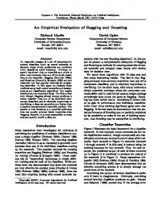
$importance Sepal.Length 0

Sepal.Width Petal.Length 0 79.69223

Petal.Width 20.30777

attr(,"class") [1] "bagging" In line with boosting, the variables with the highest contributions are Petal.Length (79.69%) and Petal.Width (20.31%). On the contrary, the contribution of the other two variables is zero. It is graphically shown in Figure 2. R> barplot(iris.bagging$imp[order(iris.bagging$imp, decreasing = TRUE)], + ylim = c(0, 100), main = "Variables Relative Importance", + col = "lightblue") The object iris.bagging can be used to compute the confusion matrix and the training set error. As can be seen, only two cases are wrongly classified (two virginica flowers classified as versicolor), therefore the error is 2.67%. R> table(iris.bagging$class, iris$Species[train], + dnn = c("Predicted Class", "Observed Class"))


17

Observed Class Predicted Class setosa versicolor virginica setosa 25 0 0 versicolor 0 25 2 virginica 0 0 23 R> 1 - sum(iris.bagging$class == iris$Species[train]) / + length(iris$Species[train]) [1] 0.02666667 In addition, predict.bagging has the same arguments and values as predict.boosting. However, it calls a fitted bagging object and returns an object of class predict.bagging. Finally, bagging.cv runs v-fold cross validation with bagging. Again, the type of v-fold cross validation is added to the arguments of the bagging function. Moreover, the output is an object of class bagging.cv similar to boosting.cv. The function predict.bagging uses the previously built object iris.bagging to predict the class for each observation in the test data set and to prune it, if necessary. The output is the same as in predict.boosting. In this case, the confusion matrix shows two virginica species classified as versicolor and vice versa, so the error is 5.33%. R> iris.predbagging iris.predbagging $formula Species ~ . $votes [,1] [,2] [,3] [1,] 9 1 0 [2,] 9 1 0 ... [26,] 1 5 4 [27,] 1 5 4 ... [74,] 0 4 6 [75,] 0 4 6 $prob [1,] [2,] ... [26,] [27,] ...

[,1] [,2] [,3] 0.9 0.1 0.9 0.1 0.1 0.1

0.5 0.5

0 0 0.4 0.4

18 [74,] [75,]

adabag: Classification with Boosting and Bagging in R 0 0

0.4 0.4

$class [1] "setosa" [6] "setosa" [11] "setosa" [16] "setosa" [21] "setosa" [26] "versicolor" [31] "versicolor" [36] "versicolor" [41] "versicolor" [46] "versicolor" [51] "virginica" [56] "virginica" [61] "virginica" [66] "virginica" [71] "virginica"

0.6 0.6

"setosa" "setosa" "setosa" "setosa" "setosa" "versicolor" "versicolor" "virginica" "versicolor" "versicolor" "virginica" "virginica" "versicolor" "virginica" "virginica"



"setosa" "setosa" "setosa" "setosa" "setosa" "versicolor" "virginica" "versicolor" "versicolor" "versicolor" "virginica" "virginica" "versicolor" "virginica" "virginica"

$confusion Observed Class Predicted Class setosa versicolor virginica setosa 25 0 0 versicolor 0 23 2 virginica 0 2 23 $error [1] 0.05333333 Next, 10-folds cross validation is applied with bagging, maintaining the number and size of the trees. In this case, there are twelve virginica species classified as versicolor and seven versicolor classified as virginica and so, the estimated error reaches 12.66%. R> iris.baggingcv iris.baggingcv $class [1] "setosa" ... [56] "virginica" [61] "versicolor" [66] "virginica" ... [136] "virginica" [141] "virginica"

"setosa"

"setosa"

"setosa"

"setosa"

"versicolor" "versicolor" "versicolor" "versicolor" "versicolor" "versicolor" "versicolor" "versicolor" "versicolor" "versicolor" "versicolor" "versicolor" "virginica" "virginica"

"virginica" "versicolor" "virginica" "versicolor" "virginica" "virginica"

Journal of Statistical Software [146] "virginica"

"virginica"

"virginica"

19

"virginica"

"virginica"

$confusion Clase real Clase estimada setosa versicolor virginica setosa 50 0 0 versicolor 0 43 12 virginica 0 7 38 $error [1] 0.1266667

3.3. The margins and errorevol functions Owing to its aforementioned importance the margins function was added to adabag to calculate the margins of a boosting or bagging classifier for a data frame as previously defined in Equation 4. Its usage is very easy with only two arguments: 1. object. This object must be the output of one of the functions bagging, boosting, predict.bagging or predict.boosting. This is assumed to be the result of some function that produces an object with at least two components named formula and class, as those returned for instance by the bagging function. 2. newdata. The same data frame used for building the object. The output, an object of class margins, is a simple list with only one vector with the margins. In the following it is shown the code to calculate the margins of the bagging classifier built in the previous section, for the training and test sets, respectively. Examples with negative margins are those which have been wrongly classified. As it was stated before, there were two and four cases in each set, respectively. R> iris.bagging.margins iris.bagging.predmargins iris.bagging.margins $margins [1] 0.8 0.8 [15] 0.8 0.8 [29] 0.1 0.1 [43] 0.1 0.1 [57] 0.2 -0.1 [71] 0.2 0.2

0.8 0.8 0.1 0.1 0.2 0.2

0.8 0.8 0.1 0.1 0.2 0.2

0.8 0.8 0.1 0.1 0.2 0.2

0.8 0.8 0.1 0.1 0.2

0.8 0.8 0.1 0.1 0.2

0.8 0.8 0.1 0.1 0.2

0.8 0.8 0.1 0.2 0.2

0.8 0.8 0.1 0.2 0.2

0.8 0.8 0.1 0.2 0.2

0.8 0.1 0.1 0.2 0.2

0.8 0.8 0.1 0.1 0.1 0.1 0.2 -0.1 0.2 0.2

0.8

0.8

0.8

0.8

0.8

0.8

0.8

0.8

R> iris.bagging.predmargins $margins [1] 0.8

0.8

0.8

0.8

0.8

0.8

20


1.0

Margin cumulative distribution graph

test

0.6 0.4 0.0

0.2

% observations

0.8

train

−1.0

−0.5

0.0

0.5

1.0

m

Figure 3: Margins for bagging in the iris example. [15] [29] [43] [57] [71]

0.8 0.1 0.1 0.2 0.2

0.8 0.1 0.1 0.2 0.2

0.8 0.1 0.1 0.2 0.2

0.8 0.1 0.1 0.2 0.2

0.8 0.8 0.8 0.1 0.1 -0.2 0.1 0.1 0.1 0.2 -0.1 0.2 0.2

0.8 0.8 0.1 -0.2 0.1 0.2 0.2 -0.1

0.8 0.1 0.2 0.2

0.8 0.1 0.2 0.2

0.1 0.1 0.2 0.2

0.1 0.1 0.2 0.2

0.1 0.1 0.2 0.2

Figure 3 shows the cumulative distribution of margins for the bagging classifier developed in this application, where the blue line corresponds to the training set and the green line to the test set. For bagging, the 2.66% of blue negative margins matches the training error and the 5.33% of the green negative ones the test error. R> R> R> + + + R> R> + R> +

margins.test R> + + R> R> +

evol.test R> R> R> R> R> R> R> R> R> R> R> + R> R> +

n R> R> + + R> R> + R> R>

data.boosting R> R> R> R> R> + R> +

data("Vehicle") l + R> +

mfinal Vehicle.adaboost 1 - sum(Vehicle.adaboost$class == Vehicle$Class[sub])/ + length(Vehicle$Class[sub]) [1] 0 R> Vehicle.adaboost.pred Vehicle.adaboost.pred$confusion Observed Class Predicted Class bus opel saab van bus 68 1 0 0 opel 1 41 22 3 saab 0 21 49 0 van 1 3 2 70 R> Vehicle.adaboost.pred$error [1] 0.1914894 R> Vehicle.SAMME 1 - sum(Vehicle.SAMME$class == Vehicle$Class[sub]) / + length(Vehicle$Class[sub]) [1] 0 R> Vehicle.SAMME.pred Vehicle.SAMME.pred$confusion Observed Class Predicted Class bus opel saab van bus 71 0 0 0 opel 1 43 24 1 saab 0 21 46 0 van 0 2 1 72 R> Vehicle.SAMME.pred$error [1] 0.177305


29

Comparing the relative importance measure for bagging and the two boosting classifiers, they agree in pointing out the two least important variables. The Max.L.Ra has the highest contribution in bagging and AdaBoost.M1 and the second one for SAMME. Figures 9, 10 and 11 show the variables ranked by its relative importance value. R> sort(Vehicle.bagging$importance, decreasing = TRUE) Max.L.Ra Sc.Var.maxis 20.06153052 11.34898853 D.Circ Scat.Ra 5.47042335 5.23492044 Kurt.maxis Kurt.Maxis 2.98563804 2.09313159

Elong 9.85195343 Circ 4.62644012 Ra.Gyr 1.70889907

Comp 8.21094638 Pr.Axis.Ra 4.32449318 Rad.Ra 1.56229729

Max.L.Rect Sc.Var.Maxis 7.90785330 5.71291406 Skew.maxis Skew.Maxis 3.84967772 3.46614732 Holl.Ra Pr.Axis.Rect 1.54524768 0.03849798

R> sort(Vehicle.adaboost$importance,decreasing = TRUE) Max.L.Ra Elong 12.0048265 8.2118048 D.Circ Sc.Var.Maxis 6.6569366 6.3137727 Kurt.maxis Skew.Maxis 4.3519975 3.6190249

Max.L.Rect 8.1391111 Comp 6.2558542 Circ 3.4026665

Pr.Axis.Ra Sc.Var.maxis Scat.Ra 7.2979696 6.8809291 6.8360291 Skew.maxis Rad.Ra Ra.Gyr 4.9731790 4.6792429 4.5205229 Kurt.Maxis Holl.Ra Pr.Axis.Rect 2.9646815 2.7585392 0.1329119

R> sort(Vehicle.SAMME$importance, decreasing = TRUE) D.Circ 8.759478 Comp 6.554652 Kurt.Maxis 4.175756

Max.L.Ra 8.373885 Rad.Ra 6.158310 Kurt.maxis 4.171116

Max.L.Rect Pr.Axis.Ra 8.216298 7.869849 Skew.Maxis Skew.maxis 5.712122 5.644969 Circ Sc.Var.maxis 3.223761 2.969842

Scat.Ra Sc.Var.Maxis 7.675569 7.190486 Ra.Gyr Elong 4.652892 4.578929 Holl.Ra Pr.Axis.Rect 2.749949 1.322136

R> barplot(sort(Vehicle.bagging$importance, decreasing = TRUE), + main = "Variables Relative Importance", col = "lightblue", + horiz = TRUE, las = 1, cex.names = .6, xlim = c(0, 20)) Figures 12, 13 and 14 show the cumulative distribution of margins for the bagging and boosting classifiers developed in this application. The margin of the training set is coloured in blue and the test set in green. For AdaBoost.M1, 19.15% of green negative margins matches the test error. For SAMME, the blue line is always positive owing to the null training error. It should also be pointed out that almost 10% of the observations in bagging, for both sets, achieve the maximum margin equal to 1, which is specially outstanding taking into account the large number of classes. To be brief only the code for one of the ensembles is shown here but all of them are available in the additional file. R> margins.train margins.test + + + R> R> + R> +

plot(sort(margins.train), (1:length(margins.train)) / length(margins.train), type = "l", xlim = c(-1,1), main = "Margin cumulative distribution graph", xlab = "m", ylab = "% observations", col = "blue3", lty = 2, lwd = 2) abline(v = 0, col = "red", lty = 2, lwd = 2) lines(sort(margins.test), (1:length(margins.test)) / length(margins.test), type = "l", cex = .5, col = "green", lwd = 2) legend("topleft", c("test", "train"), col = c("green", "blue3"), lty = 1:2, lwd = 2)

5. Summary and concluding remarks In this paper, the R package adabag consisting of eight functions is described. This package implements the AdaBoost.M1, SAMME and bagging algorithms with CART trees as base classifiers, capable of handling multiclass tasks. The ensemble trained can be used for prediction on new data using the generic predict function. Cross validation accuracy estimations can also be achieved for these classifiers. In addition, the evolution of the error as the ensemble grows can be analysed. This can help to detect overfitting and, on the other hand, if the ensemble has not been developed enough and should keep growing. In the former case, the classifier can be pruned without rebuilding it again from the start, selecting a number of iterations of the current ensemble. Furthermore, not only the predicted class is provided, but also its margin and an approximation to the probability of all the classes. The main functionalities of the package are illustrated here by applying them to three wellknown datasets from the classification literature. The similarities and differences among the three algorithms implemented in the package are also discussed. Finally, the addition of some of the plots used here to the package, with the aim of increasing the interpretability of the results, is part of the future work.

Acknowledgments The authors are very grateful to the developers of the Vehicle dataset, Pete Mowforth and Barry Shepherd from the Turing Institute, Glasgow, Scotland. Moreover, the authors would like to thank the Editors Jan de Leeuw and Achim Zeileis and two anonymous referees for their useful comments and suggestions.

References Alfaro E, Alfaro JL, G´ amez M, Garc´ıa N (2009). “A Boosting Approach for Understanding Out-of-Control Signals in Multivariate Control Charts.” International Journal of Production Research, 47(24), 6821–6834. Alfaro E, Garc´ıa N, G´ amez M, Elizondo D (2008). “Bankruptcy Forecasting: An Empirical Comparison of AdaBoost and Neural Networks.” Decission Support Systems, 45, 110–122.


33

Bache K, Lichman M (2013). “UCI Machine Learning Repository.” URL http://archive. ics.uci.edu/ml/. Banfield RE, Hall LO, Bowyer KW, Kegelmeyer WP (2007). “A Comparison of Decision Tree Ensemble Creation Techniques.” IEEE Transactions on Pattern Analysis and Machine Intelligence, 29(1), 173–180. Bauer E, Kohavi R (1999). “An Empirical Comparison of Voting Classification Algorithm: Bagging, Boosting and Variants.” Machine Learning, 36, 105–139. Breiman L (1996). “Bagging Predictors.” Machine Learning, 24(2), 123–140. Breiman L (1998). “Arcing Classifiers.” The Annals of Statistics, 26(3), 801–849. Breiman L, Friedman JH, Olshenn R, Stone CJ (1984). Classification and Regression Trees. Wadsworth International Group, Belmont. B¨ uhlmann P, Hothorn T (2007). “Boosting Algorithms: Regularization, Prediction and Model Fitting.” Statistical Science, 22(4), 477–505. Chrzanowska M, Alfaro E, Witkowska D (2009). “The Individual Borrowers Recognition: Single and Ensemble Trees.” Expert Systems with Applications, 36(3), 6409 – 6414. Culp M, Johnson K, Michailides G (2006). “ada: An R Package for Stochastic Boosting.” Journal of Statistical Software, 17(2), 1–27. URL http://www.jstatsoft.org/v17/i02/. Culp M, Johnson K, Michailidis G (2012). ada: An R Package for Stochastic Boosting. R package version 2.0-3, URL http://CRAN.R-project.org/package=ada. De Bock KW, Coussement K, Van den Poel D (2010). “Ensemble Classification Based on Generalized Additive Models.” Computational Statistics & Data Analysis, 54(6), 1535– 1546. De Bock KW, Van den Poel D (2011). “An Empirical Valuation of Rotation-Based Ensemble Classifiers for Customer Churn Prediction.” Expert Systems with Applications, 38(10), 12293–12301. ISSN 0957–4174. Dietterich T (2000). “Ensemble Methods in Machine Learning.” In Multiple Classifier Systems, volume 1857 of Lecture Notes in Computer Science, pp. 1–15. Springer-Verlag. Fan Y, Murphy TB, Watson RWG (2012). digeR: GUI Tool for Analyzing 2D DIGE Data. R package version‘1.3, URL http://CRAN.R-project.org/package=digeR. Freund Y, Schapire RE (1996). “Experiments with a New Boosting Algorithm.” In L Saitta (ed.), Proceedings of the Thirteenth International Conference on Machine Learning, pp. 148–156. Morgan Kaufmann. Freund Y, Schapire RE (1997). “A Decision-Theoretic Generalization of On-Line Learning and an Application to Boosting.” Journal of Computer and System Sciences, 55(1), 119–139. Friedman JH, Hastie T, Tibshirani R (2000). “Additive Logistic Regression: A Statistical View of Boosting.” The Annals of Statistics, 38(2), 337–407.

34


Hastie T, Tibshirani R, Friedman JH (2001). The Elements of Statistical Learning: Data Mining, Inference, and Prediction. Springer-Verlag, New York. Hothorn T (2013). “CRAN Task View: Machine Learning & Statistical Learning.” Version 2013-04-18, URL http://CRAN.R-project.org/view=MachineLearning. Hothorn T, B¨ uhlmann P, Kneib T, Schmid M, Hofner B, Sobotka F, Scheipl F (2013). mboost: Model-Based Boosting. R package version 2.2-2, URL http://CRAN.R-project. org/package=mboost. Krempl G, Hofer V (2008). “Partitioner Trees: Combining Boosting and Arbitrating.” In O Okun, G Valentini (eds.), 2nd Workshop SUEMA 2008 (ECAI 2008), pp. 61–66. Kuhn M (2008). “Building Predictive Models in R Using the caret Package.” Journal of Statistical Software, 28(5), 1–26. URL http://www.jstatsoft.org/v28/i05/. Kuhn M (2012). caret: Classification and Regression Training. R package version 5.15-023, URL http://CRAN.R-project.org/package=caret. Kuncheva LI (2004). Combining Pattern Classifiers: Methods and Algorithms. John Wiley & Sons. Leisch F, Dimitriadou E (2012). mlbench: Machine Learning Benchmark Problems. R package version 2.1-1, URL http://CRAN.R-project.org/package=mlbench. Maindonald J, Braun J (2010). Data Analysis and Graphics Using R. 3rd edition. Cambridge University Press. Mukherjee I, Schapire RE (2011). “A Theory of Multiclass Boosting.” Advances in Neural Information Processing Systems, 23(4), 1722–1722. Opitz DW, Maclin R (1999). “Popular Ensemble Methods: An Empirical Study.” Journal of Artificial Intelligence Research, 11, 169–198. R Core Team (2013). R: A Language and Environment for Statistical Computing. R Foundation for Statistical Computing, Vienna, Austria. URL http://www.R-project.org/. Ridgeway G (2013). gbm: Generalized Boosted Regression Models. R package version 2.1, URL http://CRAN.R-project.org/package=gbm. Schapire RE, Freund Y (2012). Boosting: Foundations and Algorithms. MIT, Cambridge. Schapire RE, Freund Y, Bartlett P, Lee WS (1998). “Boosting the Margin: A New Explanation for the Effectiveness of Voting Methods.” The Annals of Statistics, 26, 322–330. Stewart BM, Zhukov YM (2009). “Use of Force and Civil-Military Relations in Russia: An Automated Content Analysis.” Small Wars and Insurgencies, 20(2), 319–343. Therneau TM, Atkinson B, Ripley BD (2013). rpart: Recursive Partitioning. R package version 4.1-1, URL http://CRAN.R-project.org/package=rpart. Torgo L (2010). Data Mining with R: Learning with Case Studies. Chapman & Hall/CRC.


35

Zhu J, Zou H, Rosset S, Hastie T (2009). “Multi-Class AdaBoost.” Statistics and Its Interface, 2, 349–360.

Affiliation: Esteban Alfaro, Mat´ıas G´ amez, Noelia Garc´ıa Faculty of Economic and Business Sciences University of Castilla-La Mancha 02071 Albacete, Spain E-mail: [email protected], [email protected], [email protected]

Journal of Statistical Software published by the American Statistical Association Volume 54, Issue 2 August 2013

http://www.jstatsoft.org/ http://www.amstat.org/ Submitted: 2012-01-26 Accepted: 2013-05-29